126. Linear Quadratic Mean Field Games#
126.1. Overview#
A mean field game describes a continuum of small agents, each of whom solves a dynamic optimization problem whose payoff depends on what everybody else is doing, summarized by the cross-sectional distribution of states.
The framework was introduced by Lasry and Lions [2007] and, independently, by Huang et al. [2006].
It pairs two partial differential equations:
a Hamilton-Jacobi-Bellman equation that runs backward in time and describes an individual’s optimal choice, given paths for the aggregates
a Kolmogorov forward equation that runs forward in time and describes how the distribution of individual states evolves, given those choices
An equilibrium requires that the aggregates that agents take as given are the ones that their own decisions generate.
Readers of Rational Expectations Equilibrium will recognize that requirement: it is the “Big \(Y\), little \(y\)” idea, now applied to an entire distribution rather than to a single number.
The same pair of equations is the workhorse of continuous-time heterogeneous-agent macroeconomics; see Achdou et al. [2022].
This lecture studies a tractable special case in which the payoff is quadratic and the state evolves linearly, following Alvarez and Argente [2026].
Agents care about the cross-sectional average state \(X\), through a matrix \(\Theta_X\), and about the cross-sectional average action \(\mathcal A\), through a matrix \(\Theta_{\mathcal A}\).
The main result is a striking simplification:
Note
The equilibrium of the mean field game solves the algebraic Riccati equation of a single-agent linear quadratic regulator problem, in which the curvature matrices \(Q\) and \(\Gamma\) of the return in an agent’s own state and own action are replaced by the effective curvatures
Everything we know about the linear regulator can therefore be brought to bear on the equilibrium: existence conditions, uniqueness, comparative statics, and numerical methods.
Four lessons organize the lecture:
Effective curvature (Effective curvature). Aggregate dynamics depend on strategic interaction only through the effective curvatures, which measure how fast an agent’s marginal returns fall when everybody moves together.
Individual versus aggregate (Aggregate and individual dynamics). An agent’s deviation from the cross-sectional mean depends only on \(Q\) and \(\Gamma\), which measure how fast her marginal returns fall when she moves alone, so individual (micro) and aggregate (macro) adjustment speeds differ: three years against five in our capital example.
The missing intercept (Aggregate shocks and identification). Regressions with time effects see only deviations from the mean, while strategic interaction lives entirely in the time effects.
Marginal versus total (The planner). A planner responds to how the total return changes when everybody moves together, not to how an agent’s marginal return changes, and that can make the planner’s allocation either slower or faster than the equilibrium.
We illustrate them with two economic examples from Alvarez and Argente [2026]: an industry equilibrium with capital accumulation, and a multiproduct pricing problem with Kimball demand.
A sequel, Linear Quadratic Mean Field Games: Extensions, adds cross terms between states and actions, forcing processes, and interactions through higher moments of the cross-sectional distribution.
Riccati equations appear in several other QuantEcon lectures:
LQ Control: Foundations introduces the linear regulator and its Riccati equation
Lagrangian for LQ Control studies the state-costate system and its stable invariant subspace, which is exactly the structure we meet below
Markov Perfect Equilibrium studies dynamic games with finitely many players, where each player has a Riccati equation and the equations are coupled
A First Look at the Kalman Filter presents the Riccati equation that is dual to the control problem
Let’s start with some imports:
import numpy as np
import matplotlib.pyplot as plt
from matplotlib.patches import Patch
from matplotlib.lines import Line2D
from scipy.linalg import solve_continuous_are, expm
from scipy.optimize import brentq
126.2. The environment#
There is a continuum of agents.
An individual has state \(x \in \mathbb R^n\) and takes an action \(\alpha \in \mathbb R^k\).
The cross-sectional average state and action are
where \(m\) is the density of the state across agents and \(\alpha^*\) is the optimal policy.
The period return is
This is not the most general quadratic return.
A second-order approximation to a general return also produces cross terms between states and actions, which Linear Quadratic Mean Field Games: Extensions takes up.
It also produces terms that involve only the aggregates, which do not affect an individual’s choices but do matter for a planner, as we will see in The planner.
We omit constants, which do not affect choices, and linear terms, which affect steady-state levels but not the dynamics of deviations from them.
The individual state follows
where \(W\) is an \(n\)-dimensional Brownian motion and shocks are purely idiosyncratic for now.
Agents discount at rate \(\rho > 0\).
We assume that \(Q\) and \(\Gamma\) are positive definite, that \(\Sigma\) is positive semi-definite, that \(B\) has full row rank, and that \(\Theta_X\) and \(\Theta_{\mathcal A}\) are symmetric.
Symmetry of the interaction matrices is a genuine restriction.
The own-curvature matrix \(Q\) can always be taken to be symmetric, because \(x^\top Q x\) depends only on the symmetric part of \(Q\), but \(X^\top\Theta_X x\) pairs two different vectors, and the antisymmetric part of \(\Theta_X\) does affect choices.
It is, however, a restriction on payoffs rather than on behavior: the pricing example below has asymmetric best responses but a symmetric \(\Theta_X\).
126.2.1. Complements and substitutes#
From (126.1), the cross derivative between an agent’s own state and the average state is \(-\Theta_X\), and between her own action and the average action it is \(-\Theta_{\mathcal A}\).
So
states are strategic complements when \(-\Theta_X\) is positive definite, i.e. when \(\Theta_X\) is negative definite
states are strategic substitutes when \(\Theta_X\) is positive definite
and similarly for actions.
We compare symmetric matrices with the Loewner order, in which \(\Theta_1 \preceq \Theta_2\) means that \(\Theta_2 - \Theta_1\) is positive semi-definite.
In that order, smaller \(\Theta\) means more complementarity.
Note
The monotonicity condition that Lasry and Lions [2007] impose to obtain uniqueness corresponds here to \(\Theta_X\) being positive semi-definite, that is, to strategic substitutability in states.
We will not need it: under the symmetry assumptions above, and provided \(\Gamma + \Theta_{\mathcal A}\) is positive definite, there is at most one equilibrium whether interactions are complements or substitutes.
Linear Quadratic Mean Field Games: Extensions shows how uniqueness can fail once interactions between states and actions are allowed to be asymmetric.
126.2.2. Equilibrium#
Taking the paths \(\{X(t), \mathcal A(t)\}\) as given, an agent’s value function satisfies the HJB equation
where the Hamiltonian is
with maximizer \(\alpha^*(p,\mathcal A) = \Gamma^{-1}(B^\top p - \Theta_{\mathcal A}\mathcal A)\).
The density evolves according to the Kolmogorov forward equation
and an equilibrium is a value function, a density, and paths for \(X\) and \(\mathcal A\) that satisfy (126.3), (126.4), and the consistency requirements that \(X\) and \(\mathcal A\) really are the cross-sectional averages implied by \(m\) and by the optimal policy.
126.3. Solving the individual problem#
Given the aggregate paths, an individual faces a time-varying linear quadratic regulator problem, so her value function is quadratic:
Substituting into (126.3) and matching terms of each order gives three differential equations.
The one for \(\beta_2\) is
Notice what is absent from (126.5): neither interaction matrix appears.
The curvature of an individual’s value function is therefore the same as it would be if she were alone in the world.
Because the individual problem is concave and stationary, \(\beta_2(t)\) equals the constant \(\bar\beta_2\), the negative definite solution of
This is the familiar algebraic Riccati equation of LQ Control: Foundations, written in continuous time.
The optimal action is
Averaging across agents and solving the resulting fixed point in \(\mathcal A\) gives
Equation (126.7) is where the action interaction first bites: each agent responds to the average action, and solving for the average that is consistent with everyone doing so replaces \(\Gamma\) by \(\Gamma + \Theta_{\mathcal A}\).
126.4. A state-costate system#
Two objects now remain: the linear coefficient \(\beta_1(t)\) of the value function, and the aggregate state \(X(t)\).
Matching the terms in the HJB equation that are linear in \(x\) gives
and averaging the state equation across agents gives \(\dot X = B\mathcal A - AX\), because the idiosyncratic shocks average out.
Substituting (126.7) into both equations gives a pair of linear differential equations,
where we abbreviate
This is a state-costate system of exactly the kind studied in Lagrangian for LQ Control.
The aggregate state \(X\) has an initial condition, namely the mean of the initial distribution.
The costate \(\beta_1\) does not: it must be chosen so that the solution does not violate the agent’s transversality condition, which here requires the eigenvalues governing the path to have real parts below \(\rho/2\).
Because \(\Theta_X\), \(B\Gamma^{-1}B^\top\) and \(D\) are symmetric, \(\mathcal H - \tfrac\rho2 I\) is a Hamiltonian matrix, so its eigenvalues are symmetric about the origin.
It follows that:
Proposition 126.1
If \(\lambda\) is an eigenvalue of \(\mathcal H\), then so are \(\rho - \lambda\), \(\bar\lambda\), and \(\rho - \bar\lambda\).
So at most \(n\) eigenvalues can have real parts below \(\rho/2\), and exactly \(n\) do when none lies on the line \(\operatorname{Re}\lambda = \rho/2\).
That pins down a unique stable invariant subspace, and when \(D\) is positive definite that subspace can be written as \(\beta_1 = SX\) for a single matrix \(S\), so there is at most one equilibrium.
This is the standard connection between algebraic Riccati equations and invariant subspaces of Hamiltonian matrices, treated at length by Lancaster and Rodman [1995].
126.5. The equilibrium Riccati equation#
We look for a saddle path along which the costate is a linear function of the state, \(\beta_1(t) = S X(t)\).
Substituting into (126.8) gives a quadratic matrix equation for \(S\) whose coefficients involve \(\bar\beta_2\), and a change of variable simplifies it.
Define
The new matrix has a natural meaning.
An agent at the mean has marginal value of the state \(u_x = \beta_1 + \bar\beta_2 X = (S + \bar\beta_2)X = PX\), so \(P\) maps the aggregate state into the costate of the average agent.
Proposition 126.2
An equilibrium is characterized by a symmetric matrix \(P\) solving
with aggregate dynamics
The equilibrium requires all eigenvalues of the closed-loop matrix to have real parts below \(\rho/2\).
Compare this with the single-agent equation (126.6).
They have the same form.
The only difference is that \(Q\) has become \(Q + \Theta_X\) and \(\Gamma\) has become \(\Gamma + \Theta_{\mathcal A}\).
Proposition 126.3
Suppose \(Q + \Theta_X\) and \(\Gamma + \Theta_{\mathcal A}\) are positive definite.
Then the equilibrium of a linear quadratic mean field game with interaction matrices \(\Theta_X\) and \(\Theta_{\mathcal A}\), and its aggregate law of motion, coincide with the solution of a single-agent linear quadratic control problem whose state curvature is \(Q+\Theta_X\) and whose action curvature is \(\Gamma+\Theta_{\mathcal A}\).
This is the organizing result of the lecture.
126.5.1. Effective curvature#
We call \(Q + \Theta_X\) and \(\Gamma + \Theta_{\mathcal A}\) the effective curvatures.
They have a simple reading.
An agent’s marginal return to her state is \(-Qx - \Theta_X X\).
If she moves alone, holding \(X\) fixed, it falls with slope \(Q\).
If everybody moves together, so that \(x = X\), it equals \(-(Q + \Theta_X)X\) and falls with slope \(Q + \Theta_X\).
The first slope governs an agent’s deviations from the crowd, and the second governs the crowd.
The same reading applies to actions, with \(\Gamma\) and \(\Gamma + \Theta_{\mathcal A}\).
Fig. 126.2 below draws the two slopes for our capital accumulation example.
So strategic interaction does not change the form of the problem that determines aggregate dynamics; it changes the curvatures that enter it.
An immediate implication is that two models with very different strategic interactions can generate identical aggregate dynamics, provided their effective curvatures agree, and Aggregate shocks and identification shows what that means for estimation.
126.5.2. Existence and uniqueness#
Since \(P\) solves a standard Riccati equation, standard conditions apply.
Define
Proposition 126.4
Suppose \(B(\Gamma+\Theta_{\mathcal A})^{-1}B^\top\) is positive definite.
There is at most one equilibrium.
A necessary condition for a symmetric solution of the equilibrium Riccati equation is that \(E\) be positive semi-definite.
If \(Q + \Theta_X\) is positive definite, an equilibrium exists.
The sufficient condition has a clean reading: effective curvature must remain positive in both states and actions.
For states that is \(Q + \Theta_X \succ 0\); for actions it is the maintained assumption on \(B(\Gamma+\Theta_{\mathcal A})^{-1}B^\top\), which holds whenever \(\Gamma + \Theta_{\mathcal A} \succ 0\).
Complementarity is therefore permissible, but only up to a point.
The two interactions enter \(E\) through separate terms, and a larger \(\Theta_{\mathcal A}\) raises the second, so substitutability in actions can offset complementarity in states.
126.5.3. Aggregate and individual dynamics#
The equilibrium splits each agent’s state into the cross-sectional mean \(X\) and her deviation from it, \(z = x - X\).
Using \(\beta_1 = (P - \bar\beta_2)X\) in the optimal action shows that \(\alpha^* - \mathcal A = \Gamma^{-1}B^\top\bar\beta_2 z\).
Subtracting the aggregate law of motion from the individual one then gives
The aggregate follows the equilibrium matrix \(P\).
An agent’s deviation from the mean follows the single-agent matrix \(\bar\beta_2\), and neither interaction matrix appears, because strategic interaction operates through \(X\) and \(\mathcal A\), which drop out of deviations from the mean.
So the deviation of any agent from the crowd moves exactly as the whole economy would move if there were no interactions.
From now on we call these individual dynamics, as opposed to aggregate dynamics, and we label them “no interactions” in tables and figures.
This split is also the source of the missing intercept that we study in Aggregate shocks and identification: data on deviations from the mean reveal only the individual dynamics.
126.6. Computing equilibria#
scipy.linalg.solve_continuous_are(A, B, Q, R) returns the stabilizing solution \(\tilde P\) of
Our equation differs in two ways: our \(P\) is negative definite when the effective curvatures are positive definite, and we discount.
Writing \(P = -\tilde P\) and collecting terms shows that our equation is the standard one with \(A\) replaced by \(-(A + \tfrac\rho2 I)\).
The discount rate enters exactly as it does in the “\(\rho/2\) shift” familiar from continuous-time control.
When no admissible solution exists, solve_continuous_are usually raises an error, but not always: it can return a matrix that does not solve the equation at all.
So our function checks both the Riccati residual and the eigenvalue condition, and raises an error if either fails.
def closed_loop(A, B, Γ_eff, P):
    "The matrix governing aggregate dynamics, Ẋ = (B Γ_eff^{-1} B' P - A) X."
    return B @ np.linalg.solve(Γ_eff, B.T @ P) - A

def mfg_riccati(A, B, Q, Γ, ρ, tol=1e-8):
    """
    Solve  P B Γ^{-1} B' P = Q + ρ P + P A + A' P  for the solution P whose
    closed-loop matrix B Γ^{-1} B' P - A has eigenvalues with real parts
    below ρ/2, and raise ValueError if there is none.

    Passing Q + Θ_X and Γ + Θ_A gives the equilibrium of the mean field game;
    passing Q and Γ gives the single agent's value function curvature.
    """
    n = A.shape[0]
    try:
        P = -solve_continuous_are(-(A + ρ/2 * np.eye(n)), B, Q, Γ)
    except (np.linalg.LinAlgError, ValueError):
        raise ValueError("no admissible solution of the Riccati equation")
    quad = P @ B @ np.linalg.solve(Γ, B.T) @ P
    residual = quad - (Q + ρ*P + P @ A + A.T @ P)
    scale = 1 + np.abs(Q).max() + np.abs(quad).max()
    if (np.abs(residual).max() > tol*scale
            or np.linalg.eigvals(closed_loop(A, B, Γ, P)).real.max() >= ρ/2):
        raise ValueError("no admissible solution of the Riccati equation")
    return P
Let’s set up a two-dimensional example with complementarity in states and substitutability in actions, the configuration that Alvarez and Argente [2026] obtain from an industry equilibrium with capital accumulation.
ρ = 0.05
A = np.array([[0.4, 0.1],
              [0.0, 0.3]])
B = np.eye(2)
Q = np.array([[1.0, 0.2],
              [0.2, 0.8]])
Γ = np.array([[1.0, 0.1],
              [0.1, 1.2]])
Θ_X = np.array([[-0.3, 0.05],     # negative definite: complements in states
                [0.05, -0.2]])
Θ_A = np.array([[0.2, 0.0],       # positive definite: substitutes in actions
                [0.0, 0.1]])

β2 = mfg_riccati(A, B, Q, Γ, ρ)                 # single agent
P = mfg_riccati(A, B, Q + Θ_X, Γ + Θ_A, ρ)      # equilibrium

print("individual curvature β̄₂ =\n", β2.round(4))
print("\nequilibrium matrix P =\n", P.round(4))
individual curvature β̄₂ =
 [[-0.6614 -0.0869]
 [-0.0869 -0.654 ]]

equilibrium matrix P =
 [[-0.5353 -0.134 ]
 [-0.134  -0.5337]]
Let’s compare aggregate dynamics with individual dynamics, that is, with the dynamics of an agent’s deviation from the mean.
D = B @ np.linalg.solve(Γ + Θ_A, B.T)

U_ind = closed_loop(A, B, Γ, β2)          # individual dynamics
U_agg = closed_loop(A, B, Γ + Θ_A, P)    # aggregate dynamics

print("individual eigenvalues:", np.linalg.eigvals(U_ind).round(4))
print("aggregate eigenvalues: ", np.linalg.eigvals(U_agg).round(4))
individual eigenvalues: [-1.0698 -0.8321]
aggregate eigenvalues:  [-0.9025 -0.6423]
The aggregate eigenvalues are closer to zero, so the economy as a whole adjusts more slowly than an agent’s deviation from it.
This example has complementarity in states and substitutability in actions, and Persistence shows that both raise the sum of the eigenvalues; here each eigenvalue moves toward zero as well.
126.6.1. Checking the Hamiltonian structure#
Proposition 126.1 says the eigenvalues of \(\mathcal H\) come in pairs \(\{\lambda, \rho - \lambda\}\), and that the \(n\) eigenvalues with real parts below \(\rho/2\) are the ones that govern equilibrium dynamics.
Let’s check both claims.
BΓB = B @ np.linalg.solve(Γ, B.T)
n = A.shape[0]

Ham = np.block([[ρ*np.eye(n) + A.T - β2 @ D, Θ_X + β2 @ (BΓB - D) @ β2],
                [D,                          -A + D @ β2]])

ev = np.linalg.eigvals(Ham)
print("eigenvalues of ℋ:", np.sort(ev.real).round(4))
print("paired as λ and ρ - λ:",
      np.allclose(np.sort(ev.real), np.sort(ρ - ev.real)))

stable = np.sort(ev.real[ev.real < ρ/2])
print("\nstable half of ℋ:      ", stable.round(4))
print("closed-loop eigenvalues:", np.sort(np.linalg.eigvals(U_agg).real).round(4))
eigenvalues of ℋ: [-0.9025 -0.6423  0.6923  0.9525]
paired as λ and ρ - λ: True

stable half of ℋ:       [-0.9025 -0.6423]
closed-loop eigenvalues: [-0.9025 -0.6423]
The saddle path is the stable invariant subspace of \(\mathcal H\), exactly as in Lagrangian for LQ Control.
126.7. The scalar case#
With \(n = k = 1\) everything is explicit.
Write \(q, a, b, \gamma, \theta_X, \theta_{\mathcal A}\) for the scalars, and assume \(\gamma + \theta_{\mathcal A} > 0\).
The Riccati equation becomes a quadratic, and the admissible root gives the aggregate eigenvalue
When the initial mean \(X(0)\) is not zero, an equilibrium exists if and only if the term under the square root is positive,
and the equilibrium is stable, meaning \(\lambda<0\), if and only if
When \(q + \theta_X > 0\), as in both of our examples, formula (126.11) displays the two comparative statics at a glance.
More complementarity in states (a smaller \(\theta_X\)) raises \(\lambda\) and makes aggregate dynamics more persistent: when others stay away from the steady state, each agent has less reason to return to it.
More complementarity in actions (a smaller \(\theta_{\mathcal A}\)) lowers \(\lambda\) and makes dynamics less persistent: when others adjust, each agent wants to adjust too.
If \(q + \theta_X < 0\), the second comparative static reverses, which is why the general results below assume positive effective curvatures.
126.7.1. Four regions#
Conditions (126.12) and (126.13) define two thresholds for the state interaction,
so that \(\theta^{**} < \theta^{*}\).
As \(\theta_X\) falls, that is, as complementarity in states increases, the economy passes through four regions:
if \(\theta_X > \theta^{*}\), the equilibrium is stable and \(X(t)\) converges to zero
if \(\theta_X = \theta^{*}\), then \(\lambda = 0\) and \(X(t)\) stays where it starts
if \(\theta^{**} < \theta_X < \theta^{*}\), an equilibrium exists but \(0 < \lambda < \rho/2\), so \(X(t)\) moves away from zero, slowly enough to keep discounted payoffs finite
if \(\theta_X \leq \theta^{**}\), there is no equilibrium
So stability is lost before existence.
Formulas (126.11) to (126.13) depend on the two interactions only through the ratio \((q + \theta_X)/(\gamma + \theta_{\mathcal A})\).
In the \((\theta_X, \theta_{\mathcal A})\) plane, every curve along which that ratio is constant is a ray from the point \((-q, -\gamma)\).
So contours of the aggregate eigenvalue, the stability boundary and the existence boundary are all rays from that point.
Let’s draw them, taking a large discount rate, \(\rho = 0.5\), to widen the band between the two thresholds.
We first write the closed form, and check it against the solver.
def scalar_λ(ρ, a, b, q, γ, θ_X, θ_A):
    "Closed-form aggregate eigenvalue in the scalar case."
    return ρ/2 - np.sqrt((ρ/2 + a)**2 + b**2*(q + θ_X)/(γ + θ_A))

def half_life(λ):
    "Time for a state with eigenvalue λ < 0 to close half of a gap."
    return np.log(2)/(-λ)

ρ_s, a, b, q, γ = 0.5, 0.3, 1.0, 1.0, 1.0

errors = []
for θ_X, θ_A in ((0.0, 0.0), (-0.5, 0.0), (0.0, 0.5), (-0.5, 0.5)):
    P_s = mfg_riccati(np.array([[a]]), np.array([[b]]),
                      np.array([[q + θ_X]]), np.array([[γ + θ_A]]), ρ_s)
    λ_num = closed_loop(np.array([[a]]), np.array([[b]]),
                        np.array([[γ + θ_A]]), P_s)[0, 0]
    errors.append(abs(λ_num - scalar_λ(ρ_s, a, b, q, γ, θ_X, θ_A)))
print(f"largest gap between solver and closed form: {max(errors):.1e}")
largest gap between solver and closed form: 2.2e-16
The next figure shades the four regions and draws contours of the half-life of the aggregate state.
θ_X_grid = np.linspace(-2.0, 1.0, 400)
θ_A_grid = np.linspace(-0.99, 2.0, 400)
TX, TA = np.meshgrid(θ_X_grid, θ_A_grid)

inside = (ρ_s/2 + a)**2 + b**2*(q + TX)/(γ + TA)
λ_plane = np.where(inside >= 0, ρ_s/2 - np.sqrt(np.maximum(inside, 0)), np.nan)
region = np.where(inside < 0, 2, np.where(λ_plane >= 0, 1, 0))
hl_plane = np.where(λ_plane < 0, np.log(2)/np.abs(λ_plane), np.nan)

def θ_X_on_contour(h, θ_A):
    "The value of θ_X at which the half-life equals h, given θ_A."
    λ = -np.log(2)/h
    ratio = ((ρ_s/2 - λ)**2 - (ρ_s/2 + a)**2)/b**2
    return ratio*(γ + θ_A) - q

levels = [0.75, 1, 1.5, 2, 3, 5]
colors = ['white', '#fdd0a2', '#d9d9d9']
fig, ax = plt.subplots(figsize=(10, 5.5))
ax.contourf(TX, TA, region, levels=[-0.5, 0.5, 1.5, 2.5], colors=colors)
cs = ax.contour(TX, TA, hl_plane, levels=levels, colors='C0', linewidths=1.2)
ax.clabel(cs, fmt='%g', fontsize=9,
          manual=[(θ_X_on_contour(h, 0.6), 0.6) for h in levels])
θ_A_line = np.linspace(-γ, 2.0, 50)
ax.plot(-q - a*(a + ρ_s)*(γ + θ_A_line)/b**2, θ_A_line, 'k', lw=1.5)
ax.axhspan(-1.2, -γ, facecolor='none', hatch='//', edgecolor='grey', lw=0)
ax.plot(-q, -γ, 'ko', ms=5)
ax.annotate(r'$(-q, -\gamma)$', (-q, -γ), xytext=(-q + 0.06, -γ + 0.06))
handles = [Patch(facecolor='white', edgecolor='k', lw=0.5, label='stable'),
           Line2D([0], [0], color='k', lw=1.5, label=r'unit root, $\lambda = 0$'),
           Patch(facecolor=colors[1], label='divergent but admissible'),
           Patch(facecolor=colors[2], label='no equilibrium'),
           Patch(facecolor='none', hatch='//', edgecolor='grey',
                 label=r'excluded, $\gamma + \theta_{\mathcal{A}} \leq 0$'),
           Line2D([0], [0], color='C0', lw=1.2, label='half-life contours, years')]
ax.legend(handles=handles, loc='center left', bbox_to_anchor=(1.02, 0.5))
ax.set_xlim(-2.0, 1.0)
ax.set_ylim(-1.2, 2.0)
ax.set_xlabel(r'$\theta_X$')
ax.set_ylabel(r'$\theta_{\mathcal{A}}$')
plt.tight_layout()
plt.show()
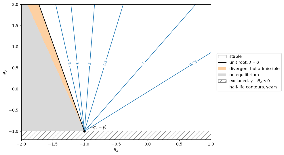
Fig. 126.1 Scalar model regions and half-lives#
Because the half-life contours are rays from \((-q, -\gamma)\), a move toward complementarity in states can be exactly offset by a move toward substitutability in actions.
The black line is the stability boundary \(\theta_X = \theta^{*}\), and the thin orange band between it and the existence boundary is the third region, in which equilibrium paths diverge.
Our solver respects the boundaries: with \(\theta_{\mathcal A} = 0\), it returns an admissible solution with \(\lambda > 0\) inside the band and raises an error beyond it.
θ_star = -q - a*(a + ρ_s)*γ/b**2
θ_2star = θ_star - (ρ_s/2)**2*γ/b**2

for θ_X in ((θ_star + θ_2star)/2, θ_2star - 0.02):
    try:
        P_s = mfg_riccati(np.array([[a]]), np.array([[b]]),
                          np.array([[q + θ_X]]), np.array([[γ]]), ρ_s)
        λ_num = closed_loop(np.array([[a]]), np.array([[b]]), np.array([[γ]]), P_s)[0, 0]
        print(f"θ_X = {θ_X:.4f}: λ = {λ_num:.4f}")
    except ValueError as e:
        print(f"θ_X = {θ_X:.4f}: {e}")
θ_X = -1.2712: λ = 0.0732
θ_X = -1.3225: no admissible solution of the Riccati equation
Exercise 126.1 asks you to derive (126.11), (126.12) and (126.13).
126.8. An industry equilibrium with capital accumulation#
The scalar model is not a toy.
Alvarez and Argente [2026] show that it describes an industry equilibrium with capital accumulation in which both kinds of interaction appear, with opposite signs.
There is a continuum of monopolistically competitive firms.
A firm with capital \(k\) produces \(y = k^\nu\) with \(0 < \nu < 1\), and a constant returns sector aggregates the differentiated goods with elasticity of substitution \(\eta > 1\).
With the final good as numeraire, a firm that produces \(y\) when industry output is \(Y\) earns revenue proportional to \(y^{1-1/\eta}Y^{1/\eta}\).
So if all other firms hold capital \(K\), operating profit is proportional to
Capital evolves according to
The firm buys investment goods at a price \(\mathcal P(I)\) that depends on aggregate investment \(I\), and it pays a convex adjustment cost \(\psi(i)\), so it chooses investment to maximize
Let \(\bar i = \delta \bar k\) be steady-state investment, normalize \(\mathcal P(\bar i) = 1\) and \(\psi'(\bar i) = 0\), and write percentage deviations from the deterministic steady state as
A second-order expansion of the return around the steady state, with the objective normalized by \(\bar\Pi \equiv \Pi(\bar k, \bar k)\), delivers exactly (126.1) with
while the state equation becomes \(dx = \delta(\alpha - x)dt + \sigma dW\) to first order, so that
Differentiating (126.14) gives closed forms:
Three features of (126.15) deserve emphasis.
First, \(\theta_X < 0\): capital stocks are strategic complements, because a larger industry capital stock raises the demand shifter \(Y^{1/\eta}\) and hence the marginal profitability of a firm’s own capital.
Second, if the supply of investment goods slopes upward then \(\mathcal P'(\bar i) > 0\) and so \(\theta_{\mathcal A} > 0\): investment rates are strategic substitutes, because everyone investing at once bids up the price of capital goods.
Third, \(q + \theta_X > 0\) for every \(\eta > 1\) and every \(\nu \in (0,1)\), so by Proposition 126.4 an equilibrium exists and is unique no matter how strong market power is and no matter how close returns to scale come to constant.
Let’s put these formulas into code, and check them against numerical derivatives of the profit function itself.
def cap_q(η, ν):
    "Own-state curvature in the capital accumulation example."
    return ν*(η - 1)/η**2*(η*(1 - ν) + ν)

def cap_θ_X(η, ν):
    "State interaction in the capital accumulation example."
    return -(η - 1)/η*ν**2/η

η_c, ν_c = 4.0, 0.7

Π = lambda k, K: k**(ν_c*(1 - 1/η_c))*K**(ν_c/η_c)

h = 1e-5
Π_kk = (Π(1+h, 1) - 2*Π(1, 1) + Π(1-h, 1))/h**2
Π_kK = (Π(1+h, 1+h) - Π(1+h, 1-h) - Π(1-h, 1+h) + Π(1-h, 1-h))/(4*h**2)

print(f"{'':>10}{'finite difference':>20}{'closed form':>15}")
print(f"{'q':>10}{-Π_kk/Π(1, 1):>20.6f}{cap_q(η_c, ν_c):>15.6f}")
print(f"{'θ_X':>10}{-Π_kK/Π(1, 1):>20.6f}{cap_θ_X(η_c, ν_c):>15.6f}")
print(f"{'q + θ_X':>10}{-(Π_kk + Π_kK)/Π(1, 1):>20.6f}"
      f"{(η_c - 1)/η_c*ν_c*(1 - ν_c):>15.6f}")
             finite difference    closed form
         q            0.249374       0.249375
       θ_X           -0.091875      -0.091875
   q + θ_X            0.157499       0.157500
The effective curvature of Effective curvature has a concrete meaning here.
The next figure plots the marginal return to a firm’s capital, measured relative to \(\bar\Pi/\bar k\), in three experiments.
In the first, one firm changes its capital while the rest of the industry stays at \(\bar k\), and the marginal return falls with slope \(-q\).
In the second, every firm changes its capital together, and the marginal return falls with the smaller slope \(-(q + \theta_X)\), because a larger industry raises the demand for each firm’s good.
The third line is the marginal revenue of the whole industry when every firm holds the same capital, \(\frac{d}{dk}\Pi(k, k) = \nu k^{\nu - 1}\).
The second line is exactly \((\eta-1)/\eta\) times the third, because a firm’s marginal revenue is only that fraction of the value of its marginal product, so the markup lowers both the level and the slope of the private return.
The third line will matter when we come to the planner.
Π_k = lambda k, K: ν_c*(1 - 1/η_c)*k**(ν_c*(1 - 1/η_c) - 1)*K**(ν_c/η_c)
k_grid = np.linspace(0.8, 1.2, 200)      # k̄ = 1, so that Π̄ = 1

fig, ax = plt.subplots(figsize=(8, 4.8))
ax.plot(k_grid, Π_k(k_grid, 1.0), lw=2,
        label=r'$\Pi_k(k, \bar k)$: one firm moves, slope $-q$')
ax.plot(k_grid, Π_k(k_grid, k_grid), lw=2,
        label=r'$\Pi_k(k, k)$: all firms move, slope $-(q+\theta_X)$')
ax.plot(k_grid, ν_c*k_grid**(ν_c - 1), lw=2, ls='--',
        label=r'$\frac{d}{dk}\Pi(k, k)$: industry, slope $-\nu(1-\nu)$')
ax.set_xlabel(r'capital relative to steady state, $k/\bar k$')
ax.set_ylabel(r'marginal return, relative to $\bar\Pi/\bar k$')
ax.set_ylim(0.45, 0.88)
ax.legend(loc='upper right')
plt.tight_layout()
plt.show()
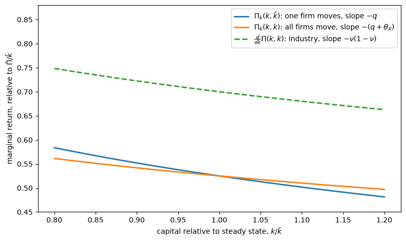
Fig. 126.2 Marginal returns to capital#
126.8.1. Calibration#
Take annual units, \(\delta = 0.10\), \(\rho = 0.05\), an elasticity of substitution \(\eta = 4\), and returns to scale \(\nu = 0.7\).
For investment costs we use a quadratic adjustment cost and a constant-elasticity supply of investment goods,
which satisfy the normalizations \(\psi'(\bar i) = 0\) and \(\mathcal P(\bar i) = 1\).
The steady-state Euler equation \(\Pi_k(\bar k, \bar k) = \rho + \delta\) gives \(\bar k^{1-\nu} = \nu(\eta-1)/[\eta(\rho+\delta)]\), and substituting into the formulas for \(\gamma\) and \(\theta_{\mathcal A}\) gives
We choose \(\phi = 1/7\), so that a firm that ignores the industry closes half of a capital gap in three years, and \(\varepsilon_s = 35/9 \approx 3.9\), a moderately elastic supply of investment goods chosen so that \(\theta_{\mathcal A} = 0.09\).
With these values \(\gamma = 0.05\).
Exercise 126.2 asks you to derive these formulas.
ρ_c, δ_c = 0.05, 0.10
φ_c, ε_s_c = 1/7, 35/9

def cap_scale(η, ν, ρ=ρ_c, δ=δ_c):
    "δ k̄^{1-ν}, which converts φ and 1/ε_s into γ and θ_A."
    return δ*ν*(η - 1)/(η*(ρ + δ))

γ_c = φ_c*cap_scale(η_c, ν_c)
θ_A_c = cap_scale(η_c, ν_c)/ε_s_c
q_c, θ_X_c = cap_q(η_c, ν_c), cap_θ_X(η_c, ν_c)

λ_c = scalar_λ(ρ_c, δ_c, δ_c, q_c, γ_c, θ_X_c, θ_A_c)

θ_star_c = -q_c - δ_c*(δ_c + ρ_c)*(γ_c + θ_A_c)/δ_c**2   # stability threshold

print(f"γ = {γ_c:.4f},  θ_A = {θ_A_c:.4f}")
print(f"q = {q_c:.4f},  θ_X = {θ_X_c:.4f},  q + θ_X = {q_c + θ_X_c:.4f}")
print(f"stability threshold θ* = {θ_star_c:.4f}")
print(f"half-life of aggregate capital = {half_life(λ_c):.2f} years")
γ = 0.0500,  θ_A = 0.0900
q = 0.2494,  θ_X = -0.0919,  q + θ_X = 0.1575
stability threshold θ* = -0.4594
half-life of aggregate capital = 4.99 years
Since the technology delivers \(q + \theta_X > 0\) and an upward-sloping supply of investment goods delivers \(\theta_{\mathcal A} > 0\), this example is always in the first of the four regions.
Complementarity in states would have to be five times stronger than the technology implies before the industry’s capital stock stopped converging.
126.8.2. How much do the interactions matter?#
Because (126.11) depends on \(\theta_X\) and \(\theta_{\mathcal A}\) separately, we can switch each interaction off and read the answer.
cases = {'no interactions':              (0.0,   0.0),
         'state complementarity only':   (θ_X_c, 0.0),
         'action substitutability only': (0.0,   θ_A_c),
         'equilibrium':                  (θ_X_c, θ_A_c)}

print(f"{'':>30}{'λ':>10}{'half-life':>12}")
for label, (tx, ta) in cases.items():
    λ_case = scalar_λ(ρ_c, δ_c, δ_c, q_c, γ_c, tx, ta)
    print(f"{label:>30}{λ_case:>10.4f}{half_life(λ_case):>12.2f}")
                                       λ   half-life
               no interactions   -0.2309        3.00
    state complementarity only   -0.1921        3.61
  action substitutability only   -0.1579        4.39
                   equilibrium   -0.1389        4.99
Both interactions slow aggregate capital adjustment, and they do so for different reasons.
Complementarity in states means that a firm has less reason to rebuild its capital while the rest of the industry is still below its steady state.
Substitutability in actions means that a burst of industry investment is expensive, so firms spread their investment over time.
Together they stretch the half-life of the industry’s capital stock from three years to five.
We will see in The planner in the capital accumulation example that a planner would adjust slightly faster than the industry does, once all the terms in the planner’s objective are counted.
126.8.3. Individual and aggregate adjustment speeds#
By (126.10), a firm’s deviation from the industry mean adjusts at the speed of a firm that ignores the industry, so the first row of the table is also the individual half-life: three years, against five for the industry, a ratio of 1.66.
Because state complementarity and action substitutability both slow aggregate adjustment here, individual capital reverts to the mean faster than aggregate capital does.
A researcher who estimated the speed of capital adjustment from firm-level data, and used it to predict the industry’s response to an industry-wide shock, would predict a half-life of three years rather than five.
That is the missing intercept of Aggregate shocks and identification at work.
The gap is a pure interaction effect: the same technology and the same adjustment costs generate both numbers.
126.8.4. Market power and returns to scale#
How does the industry’s adjustment speed depend on the two technological parameters?
Because \(\gamma\) and \(\theta_{\mathcal A}\) are measured relative to profits, they depend on \(\eta\) and \(\nu\) through \(\bar k\), so we hold the structural parameters \(\phi\) and \(\varepsilon_s\) fixed rather than \(\gamma\) and \(\theta_{\mathcal A}\).
That embeds an assumption of our calibration: the cost of a given percentage change in investment is proportional to the scale of investment \(\bar i\).
Then
in which \(\eta\) does not appear: the effective curvature and the investment costs, both measured relative to profits, are proportional to \((\eta-1)/\eta\).
So by (126.11), market power has no effect on the industry’s adjustment speed.
The invariance depends on the scaling of adjustment costs: with a cost \(\frac c2(i - \bar i)^2\) and \(c\) fixed, adjustment costs relative to profits would grow with the steady state, which rises with \(\eta\), and the industry’s half-life would rise from 4.5 years at \(\eta = 1.5\) to 5.3 years at \(\eta = 12\).
It does affect a single firm’s, because
falls as \(\eta\) rises: with more elastic demand, a firm’s revenue is closer to linear in its own capital, so its marginal return falls more slowly as it expands.
η_grid = np.linspace(1.2, 12, 200)
ν_grid = np.linspace(0.05, 0.995, 200)

def macro_micro(η, ν):
    "Aggregate and individual half-lives, holding φ and ε_s fixed."
    γ, θ_A = φ_c*cap_scale(η, ν), cap_scale(η, ν)/ε_s_c
    q, θ_X = cap_q(η, ν), cap_θ_X(η, ν)
    λ_agg = scalar_λ(ρ_c, δ_c, δ_c, q, γ, θ_X, θ_A)
    λ_ind = scalar_λ(ρ_c, δ_c, δ_c, q, γ, 0.0, 0.0)
    return half_life(λ_agg), half_life(λ_ind)

fig, axes = plt.subplots(1, 2, figsize=(11, 4.2))

hl_agg, hl_ind = np.array([macro_micro(η, ν_c) for η in η_grid]).T
axes[0].plot(η_grid, hl_agg, lw=2, label='aggregate (industry)')
axes[0].plot(η_grid, hl_ind, lw=2, ls='--', label='individual (firm)')
axes[0].set_xlabel('elasticity of substitution $\\eta$')
axes[0].set_title('varying $\\eta$, with $\\nu = 0.7$')

hl_agg, hl_ind = np.array([macro_micro(η_c, ν) for ν in ν_grid]).T
axes[1].plot(ν_grid, hl_agg, lw=2, label='aggregate (industry)')
axes[1].plot(ν_grid, hl_ind, lw=2, ls='--', label='individual (firm)')
axes[1].set_title('varying $\\nu$, with $\\eta = 4$')
axes[1].axhline(np.log(2)/δ_c, color='k', lw=1, alpha=0.6)
axes[1].set_xlabel('returns to scale $\\nu$')
axes[1].annotate('$\\ln 2/\\delta$', (0.08, np.log(2)/δ_c - 0.35))

for ax in axes:
    ax.set_ylabel('half-life in years')
    ax.legend(loc='lower right')
plt.tight_layout()
plt.show()
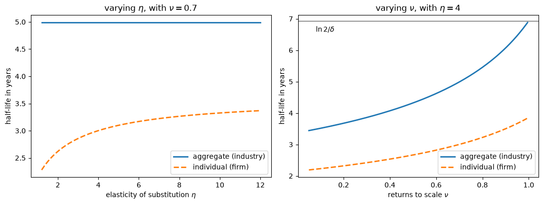
Fig. 126.3 Half-lives of industry and firm capital#
The left panel shows both results: the industry’s half-life does not move with \(\eta\), while a single firm’s rises from about 2.3 to 3.4 years as competition intensifies.
So the gap between individual and aggregate adjustment is widest when market power is greatest.
The right panel shows that both slow down as returns to scale rise.
As \(\nu\) approaches 1 the effective curvature \(q + \theta_X\) vanishes, and \(\lambda\) approaches \(-\delta\): the industry’s capital stock then returns to its steady state almost entirely through depreciation, and aggregate investment barely responds.
Fig. 126.2 shows why: as \(\nu\) approaches 1, the marginal return \(\Pi_k(k, k)\) becomes flat along the diagonal, so an industry-wide capital gap creates almost no incentive to invest differently.
Exercise 126.3 asks you to derive these results.
126.8.5. Transition paths#
Finally, let’s trace out the industry’s response to a capital stock that starts ten percent above its steady state.
Aggregate investment follows from the aggregate law of motion: \(\dot X = \delta(\mathcal A - X) = \lambda X\) gives \(\mathcal A(t) = \frac{\lambda + \delta}{\delta}X(t)\).
t_c = np.linspace(0, 25, 300)
X0_c = 0.10

fig, axes = plt.subplots(1, 2, figsize=(11, 4.2))
for label in ('no interactions', 'equilibrium'):
    tx, ta = cases[label]
    λ_case = scalar_λ(ρ_c, δ_c, δ_c, q_c, γ_c, tx, ta)
    path = X0_c*np.exp(λ_case*t_c)
    axes[0].plot(t_c, 100*path, lw=2, label=label)
    axes[1].plot(t_c, 100*(λ_case + δ_c)/δ_c*path, lw=2, label=label)

axes[0].set_ylabel('capital, % above steady state')
axes[1].set_ylabel('investment, % above steady state')
for ax in axes:
    ax.set_xlabel('years')
    ax.axhline(0, color='k', lw=0.8)
axes[0].legend()
plt.tight_layout()
plt.show()
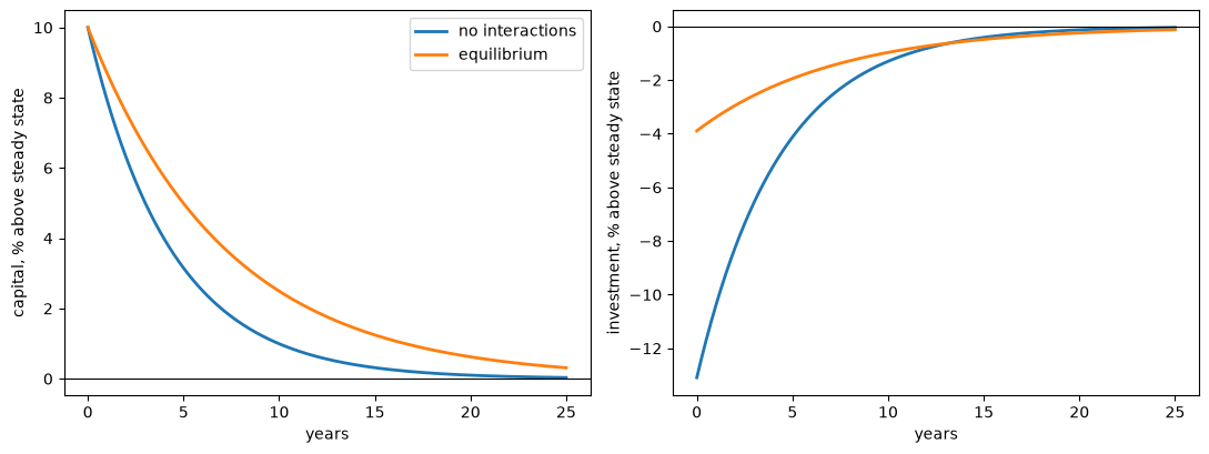
Fig. 126.4 Transition paths of capital and investment#
The right panel is the industry’s investment response, and it is where the two interactions show up most clearly.
A firm that ignored the industry would cut investment on impact by thirteen percent of its steady-state level; in equilibrium the cut is under four percent, and it is undone much more slowly.
The costate \(\beta_1(t) + \bar\beta_2 x\) that supports these paths is the marginal value of installed capital, measured as a deviation from its steady-state value; divided by the price of investment goods, it is Tobin’s marginal q, not to be confused with the curvature \(q\).
Optimal Growth Under Uncertainty and Tobin’s q studies the marginal value of capital when the irreversibility constraint \(i \geq 0\) sometimes binds, and shows that the value function remains differentiable even then; the quadratic approximation here sets that nonlinearity aside.
126.9. Aggregate shocks and identification#
Now add a shock that hits everyone at once.
Let \(\mathcal J\) be a compensated jump process, the difference between two independent Poisson processes with equal intensities, so that its increments have mean zero, and suppose
A common Brownian motion would work the same way.
With common noise the value function must keep track of the aggregate state as well as the individual state, so it becomes \(v(x, X)\).
Nevertheless, matching coefficients in the recursive HJB equation delivers a result worth emphasizing.
Proposition 126.5
With common noise, the matrix \(P\) governing aggregate dynamics solves the same equilibrium Riccati equation as before.
This is a certainty-equivalence result of the kind familiar from linear quadratic control.
The decomposition (126.10) continues to hold, with \(\Upsilon \, d\mathcal J\) added to the law of motion of \(X\), and the common shock cancels from the law of motion of an agent’s deviation \(z\).
126.9.1. The missing intercept#
Researchers often estimate how agents respond to shocks from panel data with time fixed effects, which control for aggregate conditions.
Such regressions identify how an agent responds to her position relative to others, but not the common response of all agents to an aggregate shift, which the time effects absorb; this is the “missing intercept” [Wolf, 2023].
The decomposition (126.10) makes the point exact.
Writing an agent’s action in terms of her own state and the mean gives
A regression of actions on states with time effects estimates the slope \(U_{\alpha,z}\), which contains no interaction matrix, while the time effects absorb \((U_{\alpha,X} - U_{\alpha,z})X_t\), which contains all of them.
Proposition 126.6
Data on \(x(t) - X(t)\) and \(\alpha(t)-\mathcal A(t)\) contain no information about \(\Theta_X\) or \(\Theta_{\mathcal A}\).
Note
Removing time effects from micro data removes exactly the variation that identifies strategic interaction.
To see this in the capital example, consider two industries that are identical except for the strength of complementarity in states: one has \(\theta_X = 0\), and the other has twice the calibrated amount.
Let’s compute the two policy coefficients for each.
def capital_policy(θ_X, θ_A=θ_A_c):
    "Coefficients of investment on X and on z in the capital example."
    one = np.array([[1.0]])
    P_s = mfg_riccati(δ_c*one, δ_c*one, (q_c + θ_X)*one, (γ_c + θ_A)*one, ρ_c)[0, 0]
    β2_s = mfg_riccati(δ_c*one, δ_c*one, q_c*one, γ_c*one, ρ_c)[0, 0]
    return δ_c*P_s/(γ_c + θ_A), δ_c*β2_s/γ_c

industries = (('θ_X = 0', 0.0), ('θ_X = 2 × calibrated', 2*θ_X_c))
print(f"{'':>22}{'slope on z':>12}{'slope on X':>12}")
for label, θ_X_use in industries:
    U_αX, U_αz = capital_policy(θ_X_use)
    print(f"{label:>22}{U_αz:>12.4f}{U_αX:>12.4f}")
                        slope on z  slope on X
               θ_X = 0     -1.3093     -0.5786
  θ_X = 2 × calibrated     -1.3093     -0.1752
The slope on a firm’s deviation from the mean is the same in the two industries, and only the slope on the industry mean differs.
Now let’s simulate panels of 400 firms from the two industries, using the same shocks for both.
Both start at their steady state with some dispersion across firms, and both are hit at \(t = 2\) by a common shock that lowers every firm’s capital by ten percent.
rng = np.random.default_rng(0)
N, T, dt, σ = 400, 20.0, 0.02, 0.05
steps = int(T/dt)
dW = rng.normal(size=(steps, N))*np.sqrt(dt)     # the same draws for both
x0 = 0.05*rng.normal(size=N)
t_sim = np.arange(steps)*dt

fig, axes = plt.subplots(1, 2, figsize=(11, 4.2))
deviations = []
for k, (label, θ_X_sim) in enumerate(industries):
    U_αX, U_αz = capital_policy(θ_X_sim)
    x = x0.copy()
    X_path, z_path = np.empty(steps), np.empty(steps)
    for s in range(steps):
        if s == int(2.0/dt):
            x = x - 0.10                         # common shock
        X = x.mean()
        α = U_αX*X + U_αz*(x - X)
        X_path[s], z_path[s] = X, x[0] - X
        x = x + δ_c*(α - x)*dt + σ*dW[s]
    deviations.append(z_path)
    tex_label = label.replace('θ_X', r'$\theta_X$')
    axes[0].plot(t_sim, 100*z_path, lw=2.5 - 1.5*k, ls='-' if k == 0 else '--',
                 label=tex_label)
    axes[1].plot(t_sim, 100*X_path, lw=2, label=tex_label)

axes[0].set_title("one firm's deviation from the industry mean")
axes[1].set_title('industry mean')
for ax in axes:
    ax.set_xlabel('years')
    ax.set_ylabel('percent')
    ax.legend()
plt.tight_layout()
plt.show()

print("demeaned paths identical:", np.allclose(*deviations))
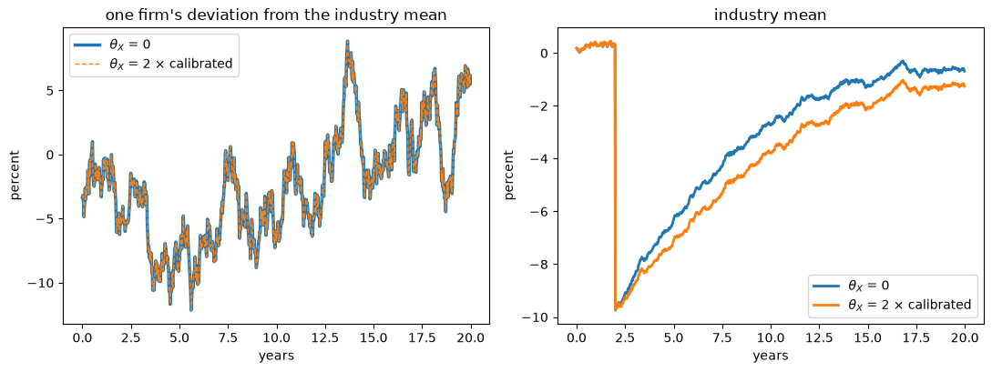
Fig. 126.5 Simulated panels from two industries#
demeaned paths identical: True
The left panel plots one firm’s deviation from its industry mean in each economy, and the two lines coincide exactly, so a regression on demeaned data would return identical estimates for the two industries.
The industry means in the right panel differ: after the common shock, the industry with stronger complementarity returns to its steady state more slowly.
The small wiggles in the industry means come from averaging the idiosyncratic shocks of only 400 firms.
The demeaned paths coincide by construction, because the slope on \(z\) does not involve \(\theta_X\), so the simulation illustrates Proposition 126.6 rather than testing it: it shows what an econometrician would see.
126.9.2. What aggregate data reveal#
Aggregate data, by contrast, do carry information about strategic interaction, and can be combined with micro data to recover it.
Collect the four reduced-form matrices that link the aggregate state, the deviations from it and the actions:
Proposition 126.7
Suppose \(\Theta_{\mathcal A}\), \(\Gamma\) and \(\rho\) are known, that \(D\) and \(\Sigma\) are nonsingular, and that \(\mathbb E[X(t)X(t)^\top]\) is nonsingular for some \(t > 0\).
If \(Q\), \(A\) and \(B\) are also known, a time series for \(X\) identifies \(\Theta_X\).
If \(B\) is also known, time series for \(X\), \(z\) and \(\mathcal A\) identify \(Q\), \(\Theta_X\) and \(A\).
If \(n = k\) and \(U_{\alpha,z} - U_{\alpha,X}\) is nonsingular, time series for \(X\), \(z\), \(\alpha\) and \(\mathcal A\) identify \(Q\), \(\Theta_X\), \(A\) and \(B\).
In every case \(\Theta_{\mathcal A}\) must be known.
Exercise 126.4 walks through the recovery, and shows why \(\Theta_X\) and \(\Theta_{\mathcal A}\) cannot be told apart without a normalization.
126.10. Persistence#
How do the interactions change aggregate adjustment when \(n > 1\)?
Throughout this section we follow Alvarez and Argente [2026] and assume that \(Q + \Theta_X\) and \(\Gamma + \Theta_{\mathcal A}\) are positive definite in every economy we compare.
As the scalar case showed, the comparative statics for actions can reverse sign without that assumption.
Proposition 126.8
Compare two economies that differ in one interaction matrix only.
More complementarity in states makes the stabilizing solution \(P\) less negative definite and raises the trace of the closed-loop matrix.
More complementarity in actions also makes \(P\) less negative definite, but lowers the trace of the closed-loop matrix.
The two kinds of interaction move \(P\) in the same direction and the trace in opposite directions because they reach the closed-loop matrix \(DP - A\) in different ways.
States act only through \(P\).
Actions also change \(D = B(\Gamma + \Theta_{\mathcal A})^{-1}B^\top\): more complementarity in actions raises \(D\), so agents respond more strongly to a given marginal value, and the net effect lowers the trace.
The trace is the sum of the eigenvalues, and also the rate at which a set of initial aggregate states contracts in volume, so in a stable equilibrium the first force slows aggregate adjustment on average and the second speeds it up.
Let’s check the first part in our two-dimensional example.
print(f"{'scale on Θ_X':>14}{'trace':>10}   eigenvalues")
for scale in (0.0, 0.5, 1.0, 1.5):
    P_s = mfg_riccati(A, B, Q + scale*Θ_X, Γ + Θ_A, ρ)
    U_s = closed_loop(A, B, Γ + Θ_A, P_s)
    print(f"{scale:>14}{np.trace(U_s):>10.4f}   {np.linalg.eigvals(U_s).real.round(4)}")
  scale on Θ_X     trace   eigenvalues
           0.0   -1.7933   [-0.9956 -0.7977]
           0.5   -1.6747   [-0.9485 -0.7262]
           1.0   -1.5448   [-0.9025 -0.6423]
           1.5   -1.3988   [-0.857  -0.5418]
Raising the scale makes \(\Theta_X\) more negative, that is, complementarity stronger, and the trace rises as claimed.
A rise in the trace says that the sum of the eigenvalues moves, not that each of them does.
Alvarez and Argente [2026] give a two-dimensional example in which a strict Loewner ordering of the Riccati solutions coexists with eigenvalues that move in opposite directions.
It sets \(\rho = 0\), holds \(D\) fixed, and compares two effective state curvatures \(Q_1\) and \(Q_2\) with \(Q_2 - Q_1\) positive definite, so that the first economy has more complementarity in states.
A_ce = np.array([[1.0, 2.0],
                 [2.0, 5.0]])
D_ce = np.array([[1.0, -3.0],
                 [-3.0, 10.0]])
Q_1 = np.array([[2.0, -1.0],
                [-1.0, 1.0]])
Q_2 = np.array([[3.0, 5.0],
                [5.0, 51.0]])

# with B = I, D = (Γ + Θ_A)^{-1}
Γ_ce = np.linalg.inv(D_ce)
P_ce = {}
for label, Q_i in (('Q_1', Q_1), ('Q_2', Q_2)):
    P_ce[label] = mfg_riccati(A_ce, np.eye(2), Q_i, Γ_ce, 0.0)
    U_i = closed_loop(A_ce, np.eye(2), Γ_ce, P_ce[label])
    print(f"{label}: trace {np.trace(U_i):.2f}, "
          f"closed-loop eigenvalues {np.sort(np.linalg.eigvals(U_i).real).round(2)}")

print("\neigenvalues of P_1 - P_2:", np.linalg.eigvalsh(P_ce['Q_1'] - P_ce['Q_2']).round(3))
print("A and D commute:", np.allclose(A_ce @ D_ce, D_ce @ A_ce))
Q_1: trace -9.57, closed-loop eigenvalues [-6.55 -3.02]
Q_2: trace -24.25, closed-loop eigenvalues [-22.68  -1.56]

eigenvalues of P_1 - P_2: [0.281 1.833]
A and D commute: False
The Riccati solutions are strictly ordered, \(P_1 \succ P_2\), and the first economy has the larger trace, as the theory requires, but only one of its eigenvalues is larger: one mode becomes more persistent and the other less.
What goes wrong is that \(A\) and \(D\) do not commute.
Since both are symmetric here, that is the same as saying that \(D^{-1}A\) is not symmetric, so the closed-loop matrix \(DP - A\) need not be similar to a symmetric matrix.
Two restrictions repair this.
Proposition 126.9
Hold \(D\) fixed and suppose that \(D^{-1}A\) is symmetric.
Then more complementarity in states raises every eigenvalue of the closed-loop matrix.
The reason is that \(DP - A = D(P - D^{-1}A)\) is similar to the symmetric matrix \(D^{1/2}(P - D^{-1}A)D^{1/2}\), whose eigenvalues rise one by one when \(P\) rises in the Loewner order.
Proposition 126.10
Suppose \(A = aI\).
Then the eigenvalues of the closed-loop matrix are real and given by
where \(\mu_j\) are the eigenvalues of \(D^{1/2}(Q+\Theta_X)D^{1/2}\).
So more complementarity in states raises every \(\lambda_j\), more complementarity in actions lowers every \(\lambda_j\), and mode \(j\) is stable if and only if \(\mu_j + a(a+\rho) > 0\).
The second result is still genuinely multidimensional.
Aggregate dynamics do decouple into scalar modes, but the coordinates that achieve this mix the eigenvectors of \(Q + \Theta_X\) and \(D\), and they differ from the coordinates that decouple individual dynamics, so the model as a whole does not separate into independent one-dimensional decisions.
Exercise 126.5 asks you to measure how often eigenvalue-by-eigenvalue monotonicity fails in random economies, and to confirm Proposition 126.9.
126.11. Multiproduct price setting with Kimball demand#
Our second example is multidimensional, and it delivers a surprise.
Alvarez and Argente [2026] study a continuum of “stores”, each selling \(n\) products with constant marginal costs \(c_j\).
Products within a store are aggregated by a CES price index with elasticity \(\bar\eta_d\), and stores are aggregated by a symmetric Kimball aggregator [Kimball, 1995].
Let \(\eta_D(y)\) be the elasticity of a store’s demand with respect to its relative price \(y\), and let \(\bar\eta_D > 1\) and \(\bar\eta_D'\) denote its level and its derivative at the symmetric point \(y = 1\).
The derivative \(\bar\eta_D'\) is the superelasticity of demand, and it is the reason Kimball demand is so widely used in models of price setting: a positive superelasticity means that a store which raises its prices above the average faces a more elastic demand, which discourages it from moving away from the crowd.
That is strategic complementarity in prices, and it is the mechanism that Klenow and Willis [2016] and much of the subsequent literature rely on for real rigidity.
Writing \(x\) and \(X\) for log deviations (equivalently, to first order, percentage deviations) of a store’s prices and of the average store’s prices from the flexible-price level \(\bar p_i = \bar c_i \bar\eta_D/(\bar\eta_D-1)\), and \(\bar s\) for the vector of steady-state expenditure shares, the curvature matrices are
Stare at the third line.
The superelasticity appears in \(Q\) and in \(\Theta_X\), but it cancels from \(Q + \Theta_X\).
By Proposition 126.2, the sum \(Q+\Theta_X\) is the only channel through which either matrix reaches aggregate dynamics.
Actions are price changes, and stores pay quadratic Rotemberg costs of changing prices.
The matrix \(\Gamma\) lets that cost depend on which bundle of prices is changed, with negative off-diagonal elements representing economies of scope in repricing of the kind emphasized by Midrigan [2011] and Alvarez and Lippi [2014].
There is no interaction through aggregate actions, so \(\Theta_{\mathcal A} = 0\).
With constant marginal costs \(A = 0\), and to obtain a nontrivial drift we follow Alvarez and Argente [2026] in letting marginal costs, and hence flexible prices, grow at a common rate \(\pi\).
Let \(\bar p_i(t)\) be the trend price, which grows at rate \(\pi\), and measure a price by its percentage deviation from trend, \(x_i = p_i/\bar p_i - 1\), and the action by the change in the price minus the change in the trend, in units of the trend price, \(\alpha_i = (\dot p_i - \dot{\bar p}_i)/\bar p_i\).
Then \(\dot x_i = \alpha_i - \pi x_i\), so \(A = \pi I\): a store that leaves its price change equal to the trend change sees its gap from trend eroded at rate \(\pi\).
def kimball(η_d, η_D, η_D_prime, s):
    "Curvature and state-interaction matrices under Kimball demand."
    s = np.asarray(s, dtype=float)
    ss = np.outer(s, s)
    Q = (η_D - 1)*((η_D - η_d + η_D_prime/(η_D - 1))*ss + η_d*np.diag(s))
    Θ_X = -η_D_prime*ss
    return Q, Θ_X

s_bar = np.array([0.5, 0.3, 0.2])       # three products, unequal shares
η_d, η_D = 6.0, 4.0                     # within-store and across-store elasticities
ρ_K, π_K = 0.04, 0.02                   # discount rate and cost inflation

n_K = len(s_bar)
A_K = π_K*np.eye(n_K)
B_K = np.eye(n_K)
Γ_K = 20.0*(np.eye(n_K) - 0.25*(np.ones((n_K, n_K)) - np.eye(n_K)))

print("Rotemberg cost matrix Γ =\n", Γ_K)
print("\neigenvalues of Γ:", np.linalg.eigvalsh(Γ_K).round(4))
Rotemberg cost matrix Γ =
 [[20. -5. -5.]
 [-5. 20. -5.]
 [-5. -5. 20.]]

eigenvalues of Γ: [10. 25. 25.]
126.11.1. The superelasticity and aggregate dynamics#
Now sweep the superelasticity across a wide range, including a negative value, and watch what changes and what does not.
print(f"{'η_D′':>6}  {'eigenvalues of Q':>28}  {'eigenvalues of Q + Θ_X':>28}")
for η_Dp in (-3.0, 0.0, 3.0, 10.0):
    Q_K, Θ_K = kimball(η_d, η_D, η_Dp, s_bar)
    print(f"{η_Dp:>6}  {str(np.linalg.eigvalsh(Q_K).round(3)):>28}"
          f"  {str(np.linalg.eigvalsh(Q_K + Θ_K).round(3)):>28}")
  η_D′              eigenvalues of Q        eigenvalues of Q + Θ_X
  -3.0           [2.598 4.5   7.482]           [3.127 4.766 7.827]
   0.0           [3.127 4.766 7.827]           [3.127 4.766 7.827]
   3.0           [3.435 5.096 8.329]           [3.127 4.766 7.827]
  10.0        [ 3.714  5.694 10.112]           [3.127 4.766 7.827]
The own-curvature matrix \(Q\) moves a great deal, and \(\Theta_X\) moves with it, but the effective curvature does not move at all.
Aggregate price dynamics are therefore invariant to the superelasticity.
print(f"{'η_D′':>6}  {'aggregate eigenvalues':>34}  {'individual eigenvalues':>34}")
for η_Dp in (-3.0, 0.0, 3.0, 10.0):
    Q_K, Θ_K = kimball(η_d, η_D, η_Dp, s_bar)
    P_K = mfg_riccati(A_K, B_K, Q_K + Θ_K, Γ_K, ρ_K)
    β2_K = mfg_riccati(A_K, B_K, Q_K, Γ_K, ρ_K)
    ev_agg = np.sort(np.linalg.eigvals(closed_loop(A_K, B_K, Γ_K, P_K)).real)
    ev_ind = np.sort(np.linalg.eigvals(closed_loop(A_K, B_K, Γ_K, β2_K)).real)
    print(f"{η_Dp:>6}  {str(ev_agg.round(4)):>34}  {str(ev_ind.round(4)):>34}")
  η_D′               aggregate eigenvalues              individual eigenvalues
  -3.0           [-0.6527 -0.4882 -0.3836]           [-0.5813 -0.4752 -0.3815]
   0.0           [-0.6527 -0.4882 -0.3836]           [-0.6527 -0.4882 -0.3836]
   3.0           [-0.6527 -0.4882 -0.3836]           [-0.7234 -0.4928 -0.3844]
  10.0           [-0.6527 -0.4882 -0.3836]           [-0.8713 -0.4966 -0.3853]
The left block of numbers is identical in every row, and the right block is not.
The superelasticity changes how an individual store behaves without changing how the industry behaves, just as market power did in the capital accumulation example.
Almost all of the movement is in a single mode, because \(\Theta_X\) is rank one and acts only through the store’s price index \(\bar s^\top x\).
The remaining modes, which involve relative prices within the store, barely move.
Because \(A_K = \pi I\), the aggregate eigenvalues are also given in closed form by Proposition 126.10, with \(\mu_j\) the eigenvalues of \((\Gamma + \Theta_{\mathcal A})^{-1}(Q + \Theta_X)\), which equal those of \(D^{1/2}(Q + \Theta_X)D^{1/2}\) when \(B = I\).
Let’s confirm that the formula matches the solver.
Q_K, Θ_K = kimball(η_d, η_D, 3.0, s_bar)
P_K = mfg_riccati(A_K, B_K, Q_K + Θ_K, Γ_K, ρ_K)
ev_solver = np.sort(np.linalg.eigvals(closed_loop(A_K, B_K, Γ_K, P_K)).real)
μ = np.linalg.eigvals(np.linalg.solve(Γ_K, Q_K + Θ_K)).real
ev_formula = np.sort(ρ_K/2 - np.sqrt((ρ_K/2 + π_K)**2 + μ))
print(f"largest gap between formula and solver: {np.abs(ev_solver - ev_formula).max():.1e}")
largest gap between formula and solver: 5.6e-16
126.11.2. Static complementarity#
It is worth seeing how much static complementarity we are varying.
Maximizing the static profit function gives the best response \(x^{*}(X) = -Q^{-1}\Theta_X X\), and Alvarez and Argente [2026] show that
We call the row sum of this matrix, \(\kappa/(1+\kappa)\), static pass-through: it is the response of a store’s prices to a uniform one percent rise in its competitors’ prices.
The next cell confirms the formula and reports pass-through for each superelasticity.
print(f"{'η_D′':>6}{'pass-through':>14}   best response matrix, first row")
for η_Dp in (-3.0, 0.0, 3.0, 10.0):
    Q_K, Θ_K = kimball(η_d, η_D, η_Dp, s_bar)
    BR = -np.linalg.solve(Q_K, Θ_K)
    κ = η_Dp/((η_D - 1)*η_D)
    BR_closed = κ/(1 + κ)*np.outer(np.ones(n_K), s_bar)
    assert np.allclose(BR, BR_closed)
    print(f"{η_Dp:>6}{BR.sum(axis=1)[0]:>14.4f}   {BR[0].round(4)}")

print("\nΘ_X symmetric:          ", np.allclose(Θ_K, Θ_K.T))
print("best response symmetric:", np.allclose(BR, BR.T))
  η_D′  pass-through   best response matrix, first row
  -3.0       -0.3333   [-0.1667 -0.1    -0.0667]
   0.0        0.0000   [0. 0. 0.]
   3.0        0.2000   [0.1  0.06 0.04]
  10.0        0.4545   [0.2273 0.1364 0.0909]

Θ_X symmetric:           True
best response symmetric: False
Static pass-through runs from \(-33\%\) to \(+45\%\) across these rows, and it changes sign with the superelasticity, yet every one of these economies has exactly the same aggregate dynamics.
Note
Stronger static complementarity need not mean more aggregate persistence.
What matters for aggregate dynamics is the effective curvature \(Q + \Theta_X\), not the interaction \(\Theta_X\) or the static best responses on their own.
Notice also that the best response matrix is not symmetric, because shares differ across products, while \(\Theta_X\) is symmetric, as promised in the description of the environment.
126.11.3. Aggregate and individual price paths#
The decomposition (126.10) splits a store’s prices into the industry average \(X\) and its own deviation \(z = x - X\).
The first follows the equilibrium matrix \(P\), the second the single-agent matrix \(\bar\beta_2\).
So the invariance we found should show up as identical paths for the industry and different paths for a store that is out of line.
t_K = np.linspace(0, 8, 200)
shock = 0.10*np.ones(n_K)      # ten percent above target, all products

fig, axes = plt.subplots(1, 2, figsize=(11, 4.2))
for k, η_Dp in enumerate((-3.0, 0.0, 3.0, 10.0)):
    Q_K, Θ_K = kimball(η_d, η_D, η_Dp, s_bar)
    P_K = mfg_riccati(A_K, B_K, Q_K + Θ_K, Γ_K, ρ_K)
    β2_K = mfg_riccati(A_K, B_K, Q_K, Γ_K, ρ_K)
    U_agg_K = closed_loop(A_K, B_K, Γ_K, P_K)
    U_ind_K = closed_loop(A_K, B_K, Γ_K, β2_K)
    agg = np.array([s_bar @ expm(U_agg_K*t) @ shock for t in t_K])
    dev = np.array([s_bar @ expm(U_ind_K*t) @ shock for t in t_K])
    label = f"$\\bar\\eta_D' = {η_Dp}$"
    # decreasing line widths, so that four coincident curves remain visible
    axes[0].plot(t_K, 100*agg, lw=6 - 1.5*k, label=label)
    axes[1].plot(t_K, 100*dev, lw=2, label=label)

axes[0].set_title('industry price index, $\\bar s^\\top X(t)$')
axes[1].set_title("one store's deviation, $\\bar s^\\top z(t)$")
for ax in axes:
    ax.set_xlabel('years')
    ax.set_ylabel('percent above target')
    ax.legend()
plt.tight_layout()
plt.show()
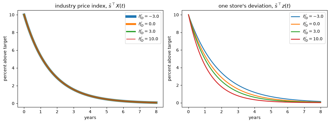
Fig. 126.6 Industry and store price paths#
The four curves in the left panel lie exactly on top of one another.
The four curves in the right panel do not: the higher the superelasticity, the faster a store closes a gap between its own prices and the industry’s.
Individual and aggregate price flexibility are governed by different objects, and only the individual one responds to the superelasticity.
126.12. The planner#
Is the equilibrium speed of adjustment efficient?
To answer, we compare it with the allocation of a utilitarian planner, who chooses an action \(\alpha(x,t)\) for every agent and date to maximize the discounted value of the cross-sectional average of the period return, subject to the Kolmogorov forward equation.
A second-order approximation to a general return also contains terms in the aggregates alone,
with \(\Lambda_X\) and \(\Lambda_{\mathcal A}\) symmetric.
An individual takes \(X\) and \(\mathcal A\) as given, so these terms do not affect her choices or the decentralized equilibrium, and we left them out of (126.1).
The planner cannot ignore them, and its period objective is
where \(X = \int x \, m(x) dx\) and \(\mathcal A = \int \alpha(x) m(x) dx\).
The planner internalizes both sides of each interaction.
Moving one agent’s state changes her own payoff and, through \(X\), everybody else’s, so the derivative of \(-X^\top\Theta_X X\) with respect to the density contributes \(-X^\top(\Theta_X + \Theta_X^\top)x\), twice what an individual takes into account.
The aggregate-only term adds \(-X^\top\Lambda_X x\), and the same reasoning applies to actions.
Proposition 126.11
Whenever the planner’s problem has a finite optimum, the planner’s allocation coincides with the decentralized equilibrium of an economy whose interaction matrices are \(\Theta_X + \Theta_X^\top + \Lambda_X\) and \(\Theta_{\mathcal A} + \Theta_{\mathcal A}^\top + \Lambda_{\mathcal A}\).
With symmetric interactions these are \(2\Theta_X + \Lambda_X\) and \(2\Theta_{\mathcal A} + \Lambda_{\mathcal A}\), and the planner’s Riccati equation is
A finite optimum exists if \(Q + 2\Theta_X + \Lambda_X\) and \(\Gamma + 2\Theta_{\mathcal A} + \Lambda_{\mathcal A}\) are positive definite.
Because each interaction matrix appears together with its transpose, the planner never needs them to be symmetric.
Symmetry is a restriction we need for the decentralized equilibrium, not for the planner.
The planner’s curvatures have a reading that complements the one in Effective curvature.
When everybody moves together, so that \(x = X\), the state part of the return including the aggregate-only term is
So \(Q + \Theta_X\) is the slope of an agent’s marginal return when everybody moves together, while \(Q + 2\Theta_X + \Lambda_X\) is the curvature of the total return when everybody moves together.
The equilibrium responds to the first and the planner to the second, and the same is true of actions.
The comparative statics of Persistence now apply directly, under the assumptions stated there.
Internalizing complementarity in states raises the trace of the closed-loop matrix, which slows aggregate adjustment on average, while internalizing complementarity in actions does the opposite.
The aggregate-only terms can reinforce or offset these forces.
A negative semi-definite \(\Lambda_X\) or a positive semi-definite \(\Lambda_{\mathcal A}\) slows adjustment further, and the opposite signs speed it up.
So the planner may adjust more slowly or more quickly than the decentralized equilibrium, and statements about individual eigenvalues need the restrictions of Proposition 126.9 or Proposition 126.10.
Our two-dimensional example has no aggregate-only terms, so we set \(\Lambda_X = \Lambda_{\mathcal A} = 0\) when we compute its planner’s allocation.
P_planner = mfg_riccati(A, B, Q + 2*Θ_X, Γ + 2*Θ_A, ρ)
U_pl = closed_loop(A, B, Γ + 2*Θ_A, P_planner)

print("individual eigenvalues:", np.sort(np.linalg.eigvals(U_ind).real).round(4))
print("aggregate eigenvalues: ", np.sort(np.linalg.eigvals(U_agg).real).round(4))
print("planner eigenvalues:   ", np.sort(np.linalg.eigvals(U_pl).real).round(4))
individual eigenvalues: [-1.0698 -0.8321]
aggregate eigenvalues:  [-0.9025 -0.6423]
planner eigenvalues:    [-0.7786 -0.4039]
With complementarity in states and substitutability in actions, both of which the planner internalizes, every planner eigenvalue is closer to zero than the corresponding equilibrium eigenvalue, so the planner’s allocation is the most persistent of the three.
Exercise 126.6 compares the planner with the equilibrium in other configurations of the interactions.
126.12.1. The planner in the capital accumulation example#
The capital accumulation example does have aggregate-only terms, and they change the answer.
Alvarez and Argente [2026] do not work out the planner for this example, so we do it here.
A second-order expansion of the firm’s return produces terms in \(K\) and \(I\) alone, which did not matter for the firm’s problem.
They are
where the second comes from the term \(\tfrac12 \bar i\,\mathcal P''(\bar i)(I - \bar i)^2\) in the expansion of investment spending \(i\,\mathcal P(I)\).
Adding the state interaction twice gives a clean result,
which is the slope of the dashed line in Fig. 126.2, the marginal revenue of the whole industry when every firm holds the same capital.
The equilibrium’s effective curvature \(\frac{\eta-1}{\eta}\nu(1-\nu)\) is smaller by the factor \((\eta-1)/\eta\).
A firm’s marginal revenue is only \((\eta-1)/\eta\) of the marginal value of its output, so an industry-wide capital gap changes the private return to investing by less than it changes the value of the industry’s output.
For actions, the constant-elasticity supply curve of the calibration gives \(\bar i\,\mathcal P''(\bar i)/\mathcal P'(\bar i) = 1/\varepsilon_s - 1\), so the planner’s action curvature is \(\gamma + (1 + 1/\varepsilon_s)\theta_{\mathcal A}\).
That exceeds the equilibrium’s \(\gamma + \theta_{\mathcal A}\), because the planner recognizes that a burst of industry investment raises the price that every firm pays.
So the two sides of the planner’s problem pull in opposite directions: on states the planner is faster than the equilibrium, on actions slower.
Let’s compute the net effect, and also what we would have found had we doubled the interactions and ignored the aggregate-only terms.
def cap_Λ_X(η, ν):
    "Aggregate-only state curvature in the capital accumulation example."
    return ν/η*(1 - ν/η)

Λ_X_c = cap_Λ_X(η_c, ν_c)
Λ_A_c = (1/ε_s_c - 1)*θ_A_c

print(f"Λ_X = {Λ_X_c:.4f},  Λ_A = {Λ_A_c:.4f}")
print(f"q + 2θ_X + Λ_X = {q_c + 2*θ_X_c + Λ_X_c:.4f},  ν(1 - ν) = {ν_c*(1 - ν_c):.4f}")

planner_cases = {'no interactions': (0.0,              0.0),
                 'equilibrium':     (θ_X_c,            θ_A_c),
                 'doubling only':   (2*θ_X_c,          2*θ_A_c),
                 'planner':         (2*θ_X_c + Λ_X_c,  2*θ_A_c + Λ_A_c)}

print(f"\n{'':>16}{'λ':>10}{'half-life':>12}{'investment on impact':>23}")
for label, (tx, ta) in planner_cases.items():
    λ_case = scalar_λ(ρ_c, δ_c, δ_c, q_c, γ_c, tx, ta)
    impact = 100*X0_c*(λ_case + δ_c)/δ_c
    print(f"{label:>16}{λ_case:>10.4f}{half_life(λ_case):>12.2f}{impact:>22.2f}%")
Λ_X = 0.1444,  Λ_A = -0.0669
q + 2θ_X + Λ_X = 0.2100,  ν(1 - ν) = 0.2100

                         λ   half-life   investment on impact
 no interactions   -0.2309        3.00                -13.09%
     equilibrium   -0.1389        4.99                 -3.89%
   doubling only   -0.1109        6.25                 -1.09%
         planner   -0.1438        4.82                 -4.38%
The last column is the change in industry investment, relative to its steady-state level, when the capital stock starts ten percent above its steady state.
At this calibration the state side wins narrowly.
The planner’s half-life is 4.8 years against the equilibrium’s 5.0, and the planner cuts investment by more on impact.
Doubling the interactions without the aggregate-only terms would have given the opposite answer, a half-life above six years.
Doubling \(\theta_X\) strengthens the complementarity in states, while \(\Lambda_X\) more than undoes it.
The next figure shows the corresponding paths of investment.
fig, ax = plt.subplots(figsize=(8, 4.5))
for label in ('equilibrium', 'doubling only', 'planner'):
    tx, ta = planner_cases[label]
    λ_case = scalar_λ(ρ_c, δ_c, δ_c, q_c, γ_c, tx, ta)
    ls = '--' if label == 'doubling only' else '-'
    ax.plot(t_c, 100*X0_c*(λ_case + δ_c)/δ_c*np.exp(λ_case*t_c), lw=2, ls=ls, label=label)
ax.axhline(0, color='k', lw=0.8)
ax.set_xlabel('years')
ax.set_ylabel('investment, % above steady state')
ax.legend()
plt.tight_layout()
plt.show()
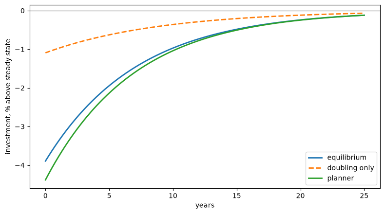
Fig. 126.7 Equilibrium and planner investment paths#
Two caveats are worth keeping in mind.
First, the planner maximizes the sum of the firms’ payoffs, so it counts the higher price of investment goods as a cost to firms; a planner who also counted the surplus of the suppliers of investment goods would treat part of it as a transfer.
Second, the comparison is local.
Within the quadratic model, the planner’s different steady state comes from linear terms, which do not affect the dynamics of deviations.
But as an approximation to the nonlinear economy, the planner’s own steady state differs from the equilibrium’s (at this calibration it has more capital), and an expansion around it would give somewhat different curvatures.
Exercise 126.7 splits the gap between the planner and the equilibrium into its state and action parts, and finds the supply elasticity at which the ranking flips.
126.12.2. The planner in the Kimball example#
Alvarez and Argente [2026] point out that in the Kimball example doubling the interaction alone would give a planner the state curvature \(Q + 2\Theta_X = (Q + \Theta_X) - \bar\eta_D' \bar s\bar s^\top\), which depends on the superelasticity, and that the aggregate-only term \(\Lambda_X\) restores the cancellation.
The reading above explains why: \(Q + 2\Theta_X + \Lambda_X\) is the curvature of a store’s profit when its prices equal the industry’s, where its relative price is one, so the superelasticity drops out, although the elasticity \(\bar\eta_D\) still matters through the markup.
With household spending held fixed, Exercise 126.8 shows that the planner’s state curvature is
against \(Q + \Theta_X = (\bar\eta_D - 1)\left[\bar\eta_D\bar s\bar s^\top + \bar\eta_d V\right]\) for the equilibrium.
The planner’s curvature is lower in the direction of a proportional increase in all of a store’s prices, which changes the store’s price level, and higher in directions that change only relative prices.
Let’s see what that does to the modes of aggregate dynamics, measuring how much each mode moves the price level by the cosine of the angle between its eigenvector and a vector of ones.
ss_bar = np.outer(s_bar, s_bar)
V = np.diag(s_bar) - ss_bar
M_act = (η_D - 1)*(ss_bar + (2*η_d - 1)*V)
Q_K, Θ_K = kimball(η_d, η_D, 3.0, s_bar)

for label, M_use in (('equilibrium', Q_K + Θ_K), ('planner', M_act)):
    U_use = closed_loop(A_K, B_K, Γ_K, mfg_riccati(A_K, B_K, M_use, Γ_K, ρ_K))
    ev, W = np.linalg.eig(U_use)
    for j in np.argsort(ev.real):
        w = W[:, j].real
        cosine = abs(w.sum())/(np.sqrt(n_K)*np.linalg.norm(w))
        print(f"{label:>12}: eigenvalue {ev[j].real:.4f}, "
              f"alignment with the price level {cosine:.2f}")
 equilibrium: eigenvalue -0.6527, alignment with the price level 0.94
 equilibrium: eigenvalue -0.4882, alignment with the price level 0.58
 equilibrium: eigenvalue -0.3836, alignment with the price level 0.37
     planner: eigenvalue -0.7001, alignment with the price level 0.07
     planner: eigenvalue -0.5372, alignment with the price level 0.10
     planner: eigenvalue -0.2959, alignment with the price level 1.00
The price-level mode is the fastest mode in equilibrium and the slowest for the planner: within the quadratic approximation, a cartel of stores would adjust its price level more slowly, and its relative prices more quickly, than the industry does.
Two qualifications apply.
This planner maximizes the stores’ joint profits and ignores the households who buy from them, so it is a collusive benchmark rather than an efficient one.
And with household spending fixed, the stores’ joint profit keeps rising as all prices rise together, so the cartel has no interior optimum and the comparison is purely local.
Exercise 126.8 also shows that with the profit normalization used to compute \(Q\) and \(\Theta_X\), which drops a factor that does not depend on the store’s own prices, the planner’s Riccati equation has no symmetric solution, so that planner’s problem has no finite optimum.
126.13. Summary#
The four lessons of the lecture, with the numbers from our examples:
Effective curvature. Aggregate dynamics solve a single-agent Riccati equation in which \(Q\) and \(\Gamma\) become \(Q + \Theta_X\) and \(\Gamma + \Theta_{\mathcal A}\); in the pricing example the superelasticity cancels from \(Q + \Theta_X\), so aggregate price dynamics do not depend on it.
Individual versus aggregate. In the capital example a firm’s deviation from the industry mean has a half-life of three years, while the industry’s capital stock has a half-life of five.
The missing intercept. In simulated panels from two industries that differ only in complementarity, the demeaned paths of firms are identical, and only the industry means differ.
Marginal versus total. The planner’s half-life in the capital example is 4.8 years, against 5.0 in equilibrium, while doubling the interactions and ignoring the aggregate-only terms would have given 6.25.
126.14. Exercises#
Exercise 126.1
This exercise derives the formulas of the scalar case.
Write the equilibrium Riccati equation in the scalar case, solve the quadratic, and show that the root satisfying the admissibility condition gives (126.11).
Derive the existence condition (126.12) and the stability condition (126.13).
With the parameters of the regions figure and \(\theta_{\mathcal A} = 0\), plot \(\lambda\) against \(\theta_X\) and mark the two thresholds.
Solution
For part 1, with \(g \equiv \gamma + \theta_{\mathcal A}\) the Riccati equation is \(\frac{b^2}{g}p^2 = q + \theta_X + (\rho + 2a)p\), and the closed-loop eigenvalue is \(\lambda = \frac{b^2}{g}p - a\).
Substituting \(p = g(\lambda + a)/b^2\) turns the Riccati equation into
a quadratic in \(\lambda\) whose roots are \(\frac\rho2 \pm \sqrt{(\frac\rho2 + a)^2 + b^2(q+\theta_X)/g}\).
The two roots are symmetric about \(\rho/2\), as Proposition 126.1 requires, and only the smaller one satisfies the admissibility condition \(\lambda < \rho/2\).
For part 2, a real root exists when the term under the square root is nonnegative, and the admissible root lies strictly below \(\rho/2\) when it is positive, which gives (126.12).
The admissible root is negative when \(\sqrt{(\rho/2 + a)^2 + b^2(q+\theta_X)/g} > \rho/2\), which after squaring gives (126.13).
For part 3, we evaluate the closed form along a line of \(\theta_X\) values, using the thresholds θ_star and θ_2star computed in the lecture.
θ_line = np.linspace(-1.30, 0.5, 400)
inside_line = (ρ_s/2 + a)**2 + b**2*(q + θ_line)/γ
λ_line = np.where(inside_line >= 0,
                  ρ_s/2 - np.sqrt(np.maximum(inside_line, 0)), np.nan)

fig, ax = plt.subplots(figsize=(8, 4.5))
ax.plot(θ_line, λ_line, lw=2)
ax.axhline(0, color='k', lw=0.8)
ax.axhline(ρ_s/2, color='grey', ls=':', lw=1, label=r'$\rho/2$')
ax.axvline(θ_star, color='r', ls='--', lw=1, label=r'$\theta^{*}$')
ax.axvline(θ_2star, color='b', ls='--', lw=1, label=r'$\theta^{**}$')
ax.set_xlabel(r'$\theta_X$')
ax.set_ylabel(r'$\lambda$')
ax.legend()
plt.tight_layout()
plt.show()
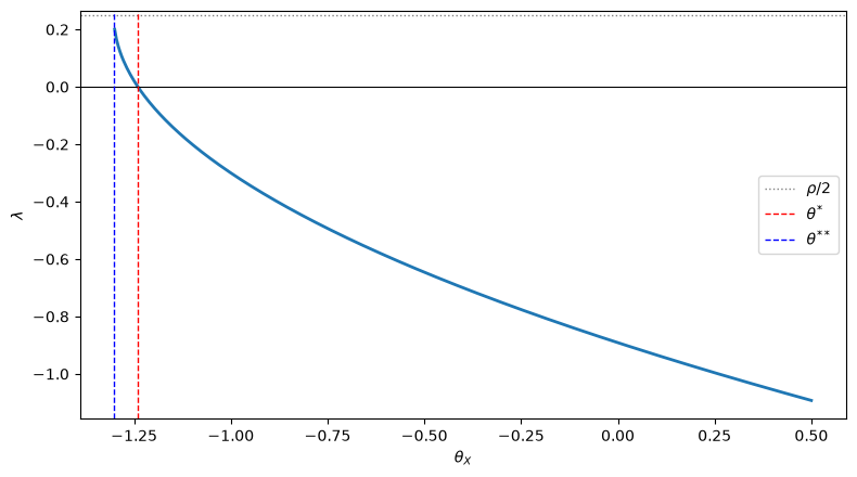
Moving left along the horizontal axis means stronger complementarity in states.
Persistence rises smoothly until \(\theta^{*}\), where the aggregate state stops converging; between \(\theta^{*}\) and \(\theta^{**}\) equilibrium paths diverge, though slowly enough to keep discounted payoffs finite; below \(\theta^{**}\) no equilibrium exists at all.
Exercise 126.2
This exercise derives the calibration of the capital accumulation example.
Use the steady-state Euler equation \(\Pi_k(\bar k, \bar k) = \rho + \delta\) to show that \(\bar k^{1-\nu} = \nu(\eta-1)/[\eta(\rho+\delta)]\), and then that \(\gamma = \phi\,\delta\bar k^{1-\nu}\) and \(\theta_{\mathcal A} = \delta \bar k^{1-\nu}/\varepsilon_s\).
Show that all pairs \((\phi, \varepsilon_s)\) with the same value of \(\phi + 1/\varepsilon_s\) generate identical aggregate dynamics, and verify numerically that they nevertheless imply different individual investment rules.
After reading The planner in the capital accumulation example, show that these pairs also imply different planner allocations.
Solution
For part 1, \(\Pi_k(k,K) = \nu\frac{\eta-1}{\eta}k^{\nu(1-1/\eta)-1}K^{\nu/\eta}\), so on the diagonal \(\Pi_k(\bar k,\bar k) = \nu\frac{\eta-1}{\eta}\bar k^{\nu-1}\).
Setting this equal to \(\rho+\delta\), which is the steady-state user cost when \(\mathcal P(\bar i) = 1\) and \(\psi'(\bar i) = 0\), gives the stated expression for \(\bar k^{1-\nu}\).
Since \(\bar\Pi = \bar k^{\nu}\), \(\bar i = \delta\bar k\), \(\psi''(\bar i) = \phi/\bar i\) and \(\mathcal P'(\bar i) = 1/(\varepsilon_s \bar i)\),
For part 2, \(\gamma + \theta_{\mathcal A} = \delta\bar k^{1-\nu}(\phi + 1/\varepsilon_s)\), and by (126.11) only this sum matters for \(\lambda\).
But the individual’s Riccati equation (126.6) involves \(\gamma\) alone, so it separates the pairs.
For part 3, the planner’s Riccati equation involves \(\gamma + 2\theta_{\mathcal A} + \Lambda_{\mathcal A} = \gamma + (1 + 1/\varepsilon_s)\theta_{\mathcal A} = \delta\bar k^{1-\nu}(\phi + 1/\varepsilon_s + 1/\varepsilon_s^2)\), so it separates them too.
The table confirms all three claims, reporting half-lives in years.
scale = cap_scale(η_c, ν_c)
print(f"{'φ':>6}{'1/ε_s':>8}{'aggregate':>12}{'individual':>12}{'planner':>10}")
for φ, inv_ε in ((0.40, 0.00), (0.30, 0.10), (1/7, 9/35), (0.05, 0.35)):
    γ_case, θ_A_case = φ*scale, inv_ε*scale
    λ_agg = scalar_λ(ρ_c, δ_c, δ_c, q_c, γ_case, θ_X_c, θ_A_case)
    λ_ind = scalar_λ(ρ_c, δ_c, δ_c, q_c, γ_case, 0.0, 0.0)
    λ_pl = scalar_λ(ρ_c, δ_c, δ_c, q_c, γ_case,
                    2*θ_X_c + Λ_X_c, (1 + inv_ε)*θ_A_case)
    print(f"{φ:>6.3f}{inv_ε:>8.3f}{half_life(λ_agg):>12.4f}"
          f"{half_life(λ_ind):>12.4f}{half_life(λ_pl):>10.4f}")
     φ   1/ε_s   aggregate  individual   planner
 0.400   0.000      4.9890      4.3909    4.6210
 0.300   0.100      4.9890      3.9967    4.6535
 0.143   0.257      4.9890      3.0016    4.8198
 0.050   0.350      4.9890      1.8601    4.9636
Aggregate dynamics are identical down to the last digit, while the individual half-life ranges from about 4.4 years to under 2.
Aggregate data alone cannot tell a congested market for capital goods from an expensive installation technology.
Data on firms’ deviations from the industry mean can, because they reveal \(\gamma\) alone, which is the mirror image of Proposition 126.6.
Exercise 126.3
This exercise derives the results in the subsection on market power and returns to scale.
Holding \(\phi\) and \(\varepsilon_s\) fixed, show that \((q + \theta_X)/(\gamma + \theta_{\mathcal A}) = (1-\nu)(\rho+\delta)/[\delta(\phi + 1/\varepsilon_s)]\) and \(q/\gamma = (\rho+\delta)[(1-\nu) + \nu/\eta]/(\phi\delta)\), and explain why market power affects individual but not aggregate adjustment.
Show that \(\lambda \to -\delta\) as \(\nu \to 1\), for every \(\eta > 1\), and that the response of aggregate investment to a capital gap, \((\lambda+\delta)/\delta\), goes to zero in the same limit. Explain the limit.
Solution
For part 1, from (126.15) and the calibration formulas,
Both numerator and denominator are proportional to \((\eta - 1)/\eta\), the ratio of a firm’s marginal revenue to the value of its marginal product.
For a single firm, \(q = e(1-e)\) with \(e = \nu(\eta-1)/\eta\) the elasticity of a firm’s revenue with respect to its own capital, so
Market power changes how fast a single firm’s marginal revenue falls as it expands alone, but along the diagonal the industry’s revenue is \(K^\nu\) whatever \(\eta\) is, and the \((\eta-1)/\eta\) factors cancel.
For part 2, \(q + \theta_X = \frac{\eta-1}{\eta}\nu(1-\nu) \to 0\), and with \(a = b = \delta\),
The aggregate law of motion gives \(\mathcal A = \frac{\lambda+\delta}{\delta}X\), which vanishes as \(\lambda \to -\delta\), as the table confirms.
print(f"{'ν':>8}{'q + θ_X':>10}{'λ':>10}{'half-life':>11}{'A/X':>9}")
for ν in (0.7, 0.9, 0.99, 0.999, 0.99999):
    γ_ν, θ_A_ν = φ_c*cap_scale(η_c, ν), cap_scale(η_c, ν)/ε_s_c
    λ_ν = scalar_λ(ρ_c, δ_c, δ_c, cap_q(η_c, ν), γ_ν, cap_θ_X(η_c, ν), θ_A_ν)
    print(f"{ν:>8}{cap_q(η_c,ν) + cap_θ_X(η_c,ν):>10.5f}{λ_ν:>10.5f}"
          f"{half_life(λ_ν):>11.3f}{(λ_ν + δ_c)/δ_c:>9.4f}")
       ν   q + θ_X         λ  half-life      A/X
     0.7   0.15750  -0.13894      4.989  -0.3894
     0.9   0.06750  -0.11419      6.070  -0.1419
    0.99   0.00743  -0.10149      6.830  -0.0149
   0.999   0.00075  -0.10015      6.921  -0.0015
 0.99999   0.00001  -0.10000      6.931  -0.0000
As \(\nu\) approaches 1 the profit function (126.14) approaches one that is homogeneous of degree one in \((k, K)\) jointly, along which \(\Pi_k(k,k)\) does not depend on \(k\).
An industry-wide capital gap then creates almost no incentive to invest differently, and the gap closes almost entirely through depreciation.
The effective curvature approaches zero, the boundary of the sufficient condition \(Q + \Theta_X \succ 0\) of Proposition 126.4, while the existence condition (126.12) continues to hold with room to spare.
The limit \(\nu = 1\) itself is not an economy we can study this way: with constant returns the steady-state Euler equation has no solution, and \(\bar k\) grows without bound as \(\nu \to 1\).
Exercise 126.4
This exercise works through the identification results of Aggregate shocks and identification.
Suppose an econometrician knows \(\rho\), \(Q\), \(A\), \(B\), \(\Gamma\) and \(\Theta_{\mathcal A}\), and estimates the aggregate drift matrix \(U_{\dot X, X}\). Show how to recover \(\Theta_X\), and verify your procedure numerically in the two-dimensional example.
In the scalar model, show that \(\theta_X\) and \(\theta_{\mathcal A}\) are not separately identified: construct a family of pairs that generate identical aggregate dynamics and identical policy coefficients.
Now suppose the econometrician knows only \(\rho\), \(\Gamma\) and \(\Theta_{\mathcal A}\), but observes \(X\), \(z\), \(\alpha\) and \(\mathcal A\), so that all four reduced-form matrices are available. Replace \(B\) by \(\begin{bmatrix} 1 & 0.3 \\ 0 & 0.8\end{bmatrix}\) in the two-dimensional example, and recover \(B\), \(A\), \(Q\) and \(\Theta_X\).
Solution
For part 1, invert the definition of the closed-loop matrix to get \(P\), then read \(\Theta_X\) off the equilibrium Riccati equation:
Let’s apply this to the aggregate drift of the two-dimensional example.
U_obs = closed_loop(A, B, Γ + Θ_A, P)      # what the econometrician estimates

P_hat = np.linalg.solve(D, U_obs + A)
Θ_X_hat = P_hat @ D @ P_hat - Q - ρ*P_hat - P_hat @ A - A.T @ P_hat

print("true Θ_X =\n", Θ_X.round(6))
print("\nrecovered Θ_X =\n", Θ_X_hat.round(6))
print(f"\nmaximum error: {np.abs(Θ_X - Θ_X_hat).max():.2e}")
true Θ_X =
 [[-0.3   0.05]
 [ 0.05 -0.2 ]]

recovered Θ_X =
 [[-0.3   0.05]
 [ 0.05 -0.2 ]]

maximum error: 1.67e-16
For part 2, formula (126.11) shows that \(\lambda\) depends on the two interactions only through the ratio \((q+\theta_X)/(\gamma+\theta_{\mathcal A})\).
Holding that ratio fixed traces out a one-parameter family of observationally equivalent economies, one of the rays in Fig. 126.1.
The policy coefficient cannot break the tie, because \(\lambda = b\,U_{\alpha,X} - a\) ties it to \(\lambda\).
ratio = (q + (-0.4))/(γ + 0.3)       # baseline θ_X = -0.4, θ_A = 0.3

print(f"{'θ_A':>7}{'θ_X':>12}{'λ':>12}{'policy coeff':>15}")
for θ_A_alt in (0.3, 0.0, 0.6, 1.0):
    θ_X_alt = ratio*(γ + θ_A_alt) - q
    λ_alt = scalar_λ(ρ_s, a, b, q, γ, θ_X_alt, θ_A_alt)
    print(f"{θ_A_alt:>7.2f}{θ_X_alt:>12.6f}{λ_alt:>12.6f}{(λ_alt + a)/b:>15.6f}")
    θ_A         θ_X           λ   policy coeff
   0.30   -0.400000   -0.624093      -0.324093
   0.00   -0.538462   -0.624093      -0.324093
   0.60   -0.261538   -0.624093      -0.324093
   1.00   -0.076923   -0.624093      -0.324093
Every row describes a different economy, with a different amount of strategic complementarity in states and in actions, yet all of them generate exactly the same aggregate dynamics and the same policy rule.
Distinguishing them requires normalizing one interaction, or bringing outside information to bear.
For part 3, the two drift matrices share \(A\), so
identifies \(B\).
Then \(A = B U_{\alpha,X} - U_{\dot X,X}\), \(P = (B^\top)^{-1}(\Gamma + \Theta_{\mathcal A})U_{\alpha,X}\) and \(\bar\beta_2 = (B^\top)^{-1}\Gamma U_{\alpha,z}\).
Finally, the single-agent Riccati equation (126.6) gives \(Q\) and the equilibrium one gives \(\Theta_X\).
B_true = np.array([[1.0, 0.3],
                   [0.0, 0.8]])
Γ_eq = Γ + Θ_A

# the reduced-form matrices the econometrician estimates
β2_true = mfg_riccati(A, B_true, Q, Γ, ρ)
P_true = mfg_riccati(A, B_true, Q + Θ_X, Γ_eq, ρ)
U_XX = closed_loop(A, B_true, Γ_eq, P_true)
U_zz = closed_loop(A, B_true, Γ, β2_true)
U_αX = np.linalg.solve(Γ_eq, B_true.T @ P_true)
U_αz = np.linalg.solve(Γ, B_true.T @ β2_true)

# recovery
B_hat = (U_zz - U_XX) @ np.linalg.inv(U_αz - U_αX)
A_hat = B_hat @ U_αX - U_XX
P_hat = np.linalg.solve(B_hat.T, Γ_eq @ U_αX)
β2_hat = np.linalg.solve(B_hat.T, Γ @ U_αz)
Q_hat = (β2_hat @ B_hat @ np.linalg.solve(Γ, B_hat.T) @ β2_hat
         - ρ*β2_hat - β2_hat @ A_hat - A_hat.T @ β2_hat)
D_hat = B_hat @ np.linalg.solve(Γ_eq, B_hat.T)
Θ_X_hat = P_hat @ D_hat @ P_hat - Q_hat - ρ*P_hat - P_hat @ A_hat - A_hat.T @ P_hat

for name, est, true in (('B', B_hat, B_true), ('A', A_hat, A),
                        ('Q', Q_hat, Q), ('Θ_X', Θ_X_hat, Θ_X)):
    print(f"maximum error in {name:>3}: {np.abs(est - true).max():.1e}")
maximum error in   B: 3.3e-16
maximum error in   A: 1.7e-16
maximum error in   Q: 6.7e-16
maximum error in Θ_X: 3.9e-16
Every object is recovered to machine precision, but only because \(\Theta_{\mathcal A}\) was known: part 2 shows that it cannot be recovered along with the rest.
Exercise 126.5
Proposition 126.8 says that stronger complementarity in states raises the trace of the closed-loop matrix, and the example of Alvarez and Argente [2026] shows that it need not raise every eigenvalue.
How common is that?
Draw many random two-dimensional economies: take \(B = I\) and \(\Theta_{\mathcal A} = 0\), let \(Q\) and \(\Gamma\) be random positive definite matrices, let \(\Theta_X\) be random negative definite, and set \(\rho = 0.05\). For each draw, compare the equilibrium with interaction \(\Theta_X\) to the one with \(1.5\,\Theta_X\), keeping only draws in which \(Q + 1.5\,\Theta_X\) is positive definite. Report how often the trace rises and how often every eigenvalue rises.
Repeat the experiment with \(A = \Gamma^{-1}S\) for a random symmetric \(S\), so that \(D^{-1}A = S\) is symmetric, and confirm Proposition 126.9.
Solution
We write one function for both experiments, taking the rule that draws \(A\) as an argument.
def compare_draws(draw_A, n_draws=400, seed=3, ρ=0.05):
    """
    Compare equilibria with interactions Θ_X and 1.5 Θ_X in random
    two-dimensional economies with B = I and Θ_A = 0.  draw_A(rng, Γ)
    returns the drift matrix.  Returns the number of draws kept, the number
    in which the trace rose and the number in which every eigenvalue rose.
    """
    rng = np.random.default_rng(seed)
    I2 = np.eye(2)
    kept = trace_rose = eig_rose = 0
    for _ in range(n_draws):
        M = rng.normal(size=(2, 2)); Q_r = M @ M.T + 0.5*I2
        M = rng.normal(size=(2, 2)); Γ_r = M @ M.T + 0.5*I2
        M = rng.normal(size=(2, 2)); Θ_r = -0.2*(M @ M.T)
        A_r = draw_A(rng, Γ_r)
        if np.linalg.eigvalsh(Q_r + 1.5*Θ_r).min() <= 0:
            continue
        J0 = closed_loop(A_r, I2, Γ_r, mfg_riccati(A_r, I2, Q_r + Θ_r, Γ_r, ρ))
        J1 = closed_loop(A_r, I2, Γ_r, mfg_riccati(A_r, I2, Q_r + 1.5*Θ_r, Γ_r, ρ))
        e0 = np.sort(np.linalg.eigvals(J0).real)
        e1 = np.sort(np.linalg.eigvals(J1).real)
        kept += 1
        trace_rose += np.trace(J1) > np.trace(J0) - 1e-10
        eig_rose += np.all(e1 >= e0 - 1e-10)
    return kept, trace_rose, eig_rose

def general_drift(rng, Γ):
    "A random drift matrix with no particular structure."
    return rng.normal(size=(2, 2))*0.3 + 0.4*np.eye(2)

def symmetric_drift(rng, Γ):
    "A random drift matrix with Γ A symmetric, so that D^{-1} A is symmetric."
    M = rng.normal(size=(2, 2))
    return np.linalg.solve(Γ, 0.3*(M + M.T) + 0.4*np.eye(2))

for label, draw_A in (('general A', general_drift), ('D⁻¹A symmetric', symmetric_drift)):
    kept, trace_rose, eig_rose = compare_draws(draw_A)
    print(f"{label:>16}: draws kept {kept}, trace rose {trace_rose}, "
          f"every eigenvalue rose {eig_rose}")
       general A: draws kept 266, trace rose 266, every eigenvalue rose 228
  D⁻¹A symmetric: draws kept 266, trace rose 266, every eigenvalue rose 266
The trace result holds in every draw, as the theory says it must.
With a general drift matrix, eigenvalue-by-eigenvalue monotonicity fails in a minority of draws.
The obstacle is that \(D^{-1}A\) need not be symmetric (here \(A\) itself is not symmetric), so the closed-loop matrix \(DP - A\) need not be similar to a symmetric matrix, and a change that slows adjustment overall can still speed it up along some direction.
When \(D^{-1}A\) is symmetric, every eigenvalue rises in every draw, as Proposition 126.9 says.
Note that \(Q + \Theta_X\) and \(D\) need not commute in either experiment: by Proposition 126.10, that kind of non-commutativity does not by itself break monotonicity.
Exercise 126.6
Compare the planner with the decentralized equilibrium in the two-dimensional example from the lecture, with no aggregate-only terms.
Compute the eigenvalues of the closed-loop matrix for the equilibrium and for the planner in four cases: only complementarity in states (\(\Theta_X\) as in the lecture, \(\Theta_{\mathcal A}=0\)); only substitutability in actions (\(\Theta_X = 0\), \(\Theta_{\mathcal A} = 0.2 I\)); only complementarity in actions (\(\Theta_X = 0\), \(\Theta_{\mathcal A} = -0.2 I\)); and complementarity in both.
In which cases is the planner’s allocation more persistent than the equilibrium? Explain.
Solution
We compute both sets of eigenvalues in each case.
def eigen_pair(Θ_X_use, Θ_A_use):
    "Closed-loop eigenvalues for the equilibrium and for the planner."
    P_eq = mfg_riccati(A, B, Q + Θ_X_use, Γ + Θ_A_use, ρ)
    P_pl = mfg_riccati(A, B, Q + 2*Θ_X_use, Γ + 2*Θ_A_use, ρ)
    e_eq = np.sort(np.linalg.eigvals(closed_loop(A, B, Γ + Θ_A_use, P_eq)).real)
    e_pl = np.sort(np.linalg.eigvals(closed_loop(A, B, Γ + 2*Θ_A_use, P_pl)).real)
    return e_eq, e_pl

zero = np.zeros((2, 2))
planner_tests = {'states, complements':  (Θ_X, zero),
                 'actions, substitutes': (zero,  0.2*np.eye(2)),
                 'actions, complements': (zero, -0.2*np.eye(2)),
                 'both complements':     (Θ_X, -0.2*np.eye(2))}

print(f"{'case':24}{'equilibrium':>22}{'planner':>22}   planner slower?")
for label, (tx, ta) in planner_tests.items():
    e_eq, e_pl = eigen_pair(tx, ta)
    slower = bool(np.all(e_pl >= e_eq - 1e-12))
    print(f"{label:24}{str(e_eq.round(4)):>22}{str(e_pl.round(4)):>22}   {slower}")
case                               equilibrium               planner   planner slower?
states, complements          [-0.9584 -0.673 ]     [-0.8522 -0.4287]   True
actions, substitutes         [-0.9933 -0.7741]     [-0.9344 -0.7284]   True
actions, complements         [-1.1748 -0.9088]     [-1.3325 -1.0151]   False
both complements             [-1.0426 -0.7346]     [-1.0137 -0.4958]   True
With only complementarity in states, the planner’s allocation is more persistent.
The planner recognizes that when one agent stays away from the steady state, others are content to stay away too, so there is less reason to hurry back.
With only substitutability in actions the planner is also slower, because it recognizes that a burst of adjustment by everyone at once is costly.
With only complementarity in actions the comparison reverses and the planner adjusts faster: it internalizes that when one agent adjusts, others want to adjust as well.
When complementarity is present in both states and actions, the two forces work against each other.
In this calibration the state interaction dominates and the planner is still slower, but that ranking is a quantitative accident, not a theorem.
Exercise 126.7
In The planner in the capital accumulation example the planner adjusts slightly faster than the equilibrium, because the state side and the action side of its problem pull in opposite directions.
Compute the planner’s half-life when only the state side is corrected, with state curvature \(q + 2\theta_X + \Lambda_X\) and action curvature \(\gamma + \theta_{\mathcal A}\), and when only the action side is corrected, with \(q + \theta_X\) and \(\gamma + (1 + 1/\varepsilon_s)\theta_{\mathcal A}\).
Hold \(\phi\) fixed and let the supply elasticity \(\varepsilon_s\) vary. Find the elasticity at which the planner and the equilibrium have the same half-life.
Repeat part 2 for \(\eta \in \{2, 4, 8\}\) and explain how the threshold depends on market power.
Solution
For part 1, we switch on one side of the planner’s problem at a time.
sides = {'equilibrium':      (θ_X_c,           θ_A_c),
         'state side only':  (2*θ_X_c + Λ_X_c, θ_A_c),
         'action side only': (θ_X_c,           2*θ_A_c + Λ_A_c),
         'planner':          (2*θ_X_c + Λ_X_c, 2*θ_A_c + Λ_A_c)}

for label, (tx, ta) in sides.items():
    λ_case = scalar_λ(ρ_c, δ_c, δ_c, q_c, γ_c, tx, ta)
    print(f"{label:>18}: half-life {half_life(λ_case):.2f} years")
       equilibrium: half-life 4.99 years
   state side only: half-life 4.62 years
  action side only: half-life 5.17 years
           planner: half-life 4.82 years
On its own, the state side would cut the half-life to 4.6 years and the action side would raise it to 5.2 years.
For parts 2 and 3, we write the gap between the two half-lives as a function of \(1/\varepsilon_s\) and find its root.
def planner_gap(inv_ε, η):
    "Planner's half-life minus the equilibrium's, as a function of 1/ε_s."
    scale_η = cap_scale(η, ν_c)
    γ_η, θ_A_η = φ_c*scale_η, inv_ε*scale_η
    q_η, θ_X_η = cap_q(η, ν_c), cap_θ_X(η, ν_c)
    λ_eq = scalar_λ(ρ_c, δ_c, δ_c, q_η, γ_η, θ_X_η, θ_A_η)
    λ_pl = scalar_λ(ρ_c, δ_c, δ_c, q_η, γ_η,
                         2*θ_X_η + cap_Λ_X(η, ν_c), (1 + inv_ε)*θ_A_η)
    return half_life(λ_pl) - half_life(λ_eq)

for η in (2.0, 4.0, 8.0):
    inv_star = brentq(planner_gap, 0.01, 20.0, args=(η,))
    print(f"η = {η}: half-lives coincide at ε_s = {1/inv_star:.2f}")
η = 2.0: half-lives coincide at ε_s = 0.89
η = 4.0: half-lives coincide at ε_s = 2.27
η = 8.0: half-lives coincide at ε_s = 4.33
With \(\eta = 4\), the planner is faster whenever the supply of investment goods is more elastic than about 2.3, which includes the calibrated 3.9, and slower when it is less elastic.
The threshold rises with \(\eta\).
The planner’s advantage on the state side is \(\nu(1-\nu) - \frac{\eta-1}{\eta}\nu(1-\nu) = \nu(1-\nu)/\eta\), which shrinks as market power falls.
So in a more competitive industry, a smaller penalty on the action side, which means a more elastic supply of investment goods, is enough to make the planner slower.
Exercise 126.8
This exercise derives the planner’s state curvature in the Kimball example, and checks it against the profit function itself.
Normalize flexible prices to one, so that the CES weights equal the expenditure shares \(\bar s\) and marginal costs equal \((\bar\eta_D - 1)/\bar\eta_D\), and use a Kimball demand whose elasticity at relative price \(y\) is \(\bar\eta_D + \bar\eta_D'(y-1)\).
Let \(\Phi(p)\) be the CES price index of a store that charges prices \(p\), let \(\tilde p\) be the other stores’ prices, and let \(\mathcal Y\) be household spending, which we hold fixed.
A store’s actual profits are proportional to \(\mathcal Y/\Phi(\tilde p)\); Alvarez and Argente [2026] drop this factor, which does not depend on the store’s own prices, when they compute \(Q\) and \(\Theta_X\).
Define
so that \(\ell\) is the log of the store’s price index.
Show that along the diagonal, where a store’s prices equal the industry’s, actual profit is proportional to \(1 - \frac{\bar\eta_D-1}{\bar\eta_D}e^{(\bar\eta_d - 1)\ell(X)}\sum_j\bar s_j e^{-\bar\eta_d X_j}\), and that profit with the factor dropped is proportional to \(e^{\ell(X)}\) times that expression.
Using \(\nabla\ell(0) = \bar s\) and \(\nabla^2\ell(0) = (1 - \bar\eta_d)V\), show that \(Q + 2\Theta_X + \Lambda_X\) equals \((\bar\eta_D - 1)[\bar s\bar s^\top + (2\bar\eta_d - 1)V]\) with actual profits and \([\bar\eta_d(2\bar\eta_D - 1) - \bar\eta_D]V - \bar\eta_D\bar s\bar s^\top\) with the factor dropped.
Check both formulas, and the formulas for \(Q\) and \(\Theta_X\), against finite-difference Hessians of the profit function, for several values of the superelasticity.
Using \(V\mathbb{1} = 0\), where \(\mathbb{1}\) is a vector of ones, show that the first matrix is positive definite whenever \(\bar\eta_d > 1/2\) and the second is not positive definite. Use the matrix \(E\) of (126.9) to show that with the factor dropped the planner’s Riccati equation has no symmetric solution.
Compare the planner’s curvature with the equilibrium’s, \(Q + \Theta_X = (\bar\eta_D - 1)[\bar\eta_D\bar s\bar s^\top + \bar\eta_d V]\), in the direction \(\mathbb{1}\) and in directions \(v\) with \(\bar s^\top v = 0\).
Solution
For part 1, along the diagonal the relative price \(\Phi(p)/\Phi(\tilde p)\) equals one, so the Kimball demand function is evaluated at a constant.
Revenue from the store’s products is \(\sum_j p_j \bar s_j (p_j/\Phi(p))^{-\bar\eta_d} = \Phi(p)^{\bar\eta_d}\sum_j \bar s_j p_j^{1-\bar\eta_d} = \Phi(p) = e^{\ell(X)}\), and costs are \(\frac{\bar\eta_D-1}{\bar\eta_D}e^{\bar\eta_d\ell(X)}\sum_j\bar s_j e^{-\bar\eta_d X_j}\).
Dividing by \(\Phi(\tilde p) = e^{\ell(X)}\) gives actual profit.
For part 2, let \(g(X) = \sum_j\bar s_j e^{-\bar\eta_d X_j}\), so that \(\log g\) has gradient \(-\bar\eta_d\bar s\) and Hessian \(\bar\eta_d^2 V\) at zero.
For any function \(f\) with \(f(0) = 0\), the Hessian of \(e^{f}\) at zero is \(\nabla f\nabla f^\top + \nabla^2 f\).
For \(e^{(\bar\eta_d - 1)\ell}g\), the logarithm has gradient \((\bar\eta_d - 1)\bar s - \bar\eta_d\bar s = -\bar s\) and Hessian \((\bar\eta_d - 1)(1-\bar\eta_d)V + \bar\eta_d^2 V = (2\bar\eta_d - 1)V\), so its Hessian is \(\bar s\bar s^\top + (2\bar\eta_d - 1)V\).
For \(e^{\ell}\), the Hessian is \(\bar s\bar s^\top + (1-\bar\eta_d)V\), and for \(e^{\bar\eta_d\ell}g\) the logarithm has gradient zero and Hessian \(\bar\eta_d(1 - \bar\eta_d)V + \bar\eta_d^2V = \bar\eta_d V\).
Both profit functions equal \(1/\bar\eta_D\) at zero, and dividing the negative Hessians by that value gives the two matrices.
For part 3, we write the profit function and a finite-difference Hessian.
def hessian(f, v, h=1e-4):
    "Central finite-difference Hessian of the scalar function f at v."
    m = len(v)
    E = h*np.eye(m)
    hess = np.empty((m, m))
    for i in range(m):
        for j in range(m):
            hess[i, j] = (f(v + E[i] + E[j]) - f(v + E[i] - E[j])
                          - f(v - E[i] + E[j]) + f(v - E[i] - E[j]))/(4*h**2)
    return hess

def store_profit(x, X, η_d, η_D, η_Dp, s, actual=True):
    """
    Profit of a store charging log prices x when all other stores charge X,
    with flexible prices normalized to one.  With actual=False the factor
    𝒴/Φ(p̃), which does not depend on x, is dropped.
    """
    p, p_others = np.exp(x), np.exp(X)
    Φ = lambda p: (s @ p**(1 - η_d))**(1/(1 - η_d))
    y = Φ(p)/Φ(p_others)
    demand = y**(η_Dp - η_D)*np.exp(-η_Dp*(y - 1))
    mc = (η_D - 1)/η_D
    profit = np.sum((p - mc)*s*(p/Φ(p))**(-η_d))*demand
    return profit/Φ(p_others) if actual else profit

def profit_curvatures(η_d, η_D, η_Dp, s, actual=True):
    "Q, Θ_X and Λ_X from the Hessian of store profits at the steady state."
    n = len(s)
    f = lambda v: store_profit(v[:n], v[n:], η_d, η_D, η_Dp, s, actual)
    v0 = np.zeros(2*n)
    hess = -hessian(f, v0)/f(v0)
    return hess[:n, :n], hess[:n, n:], hess[n:, n:]
Now we compare the finite differences with the closed forms.
M_norm = (η_d*(2*η_D - 1) - η_D)*V - η_D*ss_bar

for actual, M_closed in ((True, M_act), (False, M_norm)):
    label = "actual" if actual else "factor dropped"
    for η_Dp in (-3.0, 3.0, 10.0):
        Q_f, Θ_f, Λ_f = profit_curvatures(η_d, η_D, η_Dp, s_bar, actual)
        Q_K, Θ_K = kimball(η_d, η_D, η_Dp, s_bar)
        err_QΘ = max(np.abs(Q_f - Q_K).max(), np.abs(Θ_f - Θ_K).max())
        err_M = np.abs(Q_f + 2*Θ_f + Λ_f - M_closed).max()
        print(f"{label:>15}, η_D′ = {η_Dp:>5}: error in Q and Θ_X {err_QΘ:.0e}, "
              f"error in Q + 2Θ_X + Λ_X {err_M:.0e}")
         actual, η_D′ =  -3.0: error in Q and Θ_X 1e-06, error in Q + 2Θ_X + Λ_X 7e-07
         actual, η_D′ =   3.0: error in Q and Θ_X 9e-07, error in Q + 2Θ_X + Λ_X 6e-07
         actual, η_D′ =  10.0: error in Q and Θ_X 9e-07, error in Q + 2Θ_X + Λ_X 7e-07
 factor dropped, η_D′ =  -3.0: error in Q and Θ_X 1e-06, error in Q + 2Θ_X + Λ_X 6e-07
 factor dropped, η_D′ =   3.0: error in Q and Θ_X 9e-07, error in Q + 2Θ_X + Λ_X 5e-07
 factor dropped, η_D′ =  10.0: error in Q and Θ_X 9e-07, error in Q + 2Θ_X + Λ_X 6e-07
The formulas hold for every superelasticity, and neither planner matrix depends on it.
Dropping the factor leaves \(Q\) and \(\Theta_X\) unchanged, because the store’s first-order condition holds at the steady state, but it changes \(\Lambda_X\).
For part 4, \(v^\top V v = \sum_j\bar s_j v_j^2 - (\bar s^\top v)^2 \geq 0\), with equality only when \(v\) is proportional to \(\mathbb{1}\), and then \(v^\top\bar s\bar s^\top v > 0\).
So the actual matrix is positive definite whenever \(2\bar\eta_d - 1 > 0\).
With household spending fixed, an industry-wide price increase lowers quantities, so joint profit is concave in the level of prices.
For the other matrix, \(V\mathbb{1} = 0\) and \(\bar s^\top\mathbb{1} = 1\) give \(\mathbb{1}^\top M\mathbb{1} = -\bar\eta_D < 0\).
Dropping the factor holds quantities fixed, so raising all prices in proportion raises profit at an increasing rate.
The planner’s problem has \(\Gamma + 2\Theta_{\mathcal A} + \Lambda_{\mathcal A} = \Gamma\), so its version of \(E\) is \(M + (\pi + \rho/2)^2\Gamma\).
for label, M_closed in (('actual', M_act), ('factor dropped', M_norm)):
    E_pl = M_closed + (π_K + ρ_K/2)**2*Γ_K
    print(f"{label:>15}: eigenvalues of E {np.linalg.eigvalsh(E_pl).round(3)}")
    try:
        mfg_riccati(A_K, B_K, M_closed, Γ_K, ρ_K)
        print(" "*17 + "the planner's Riccati equation has an admissible solution")
    except ValueError as e:
        print(" "*17 + str(e))
         actual: eigenvalues of E [ 1.001  7.747 12.948]
                 the planner's Riccati equation has an admissible solution
 factor dropped: eigenvalues of E [-1.336  8.795 14.677]
                 no admissible solution of the Riccati equation
With the factor dropped, \(E\) has a negative eigenvalue, so by Proposition 126.4 no symmetric solution exists, the planner’s problem has no finite optimum, and our solver duly raises an error.
For part 5, the equilibrium’s curvature in the direction \(\mathbb{1}\) is \((\bar\eta_D - 1)\bar\eta_D\), against \(\bar\eta_D - 1\) for the planner, smaller by the factor \(\bar\eta_D\).
A single store that raises its prices loses customers to other stores at elasticity \(\bar\eta_D\), while stores that raise their prices together keep their revenue and only save on costs.
In directions with \(\bar s^\top v = 0\), which leave the store’s price index unchanged, the equilibrium’s curvature is \((\bar\eta_D - 1)\bar\eta_d\, v^\top\operatorname{diag}(\bar s)v\) and the planner’s is \((\bar\eta_D - 1)(2\bar\eta_d - 1)\, v^\top\operatorname{diag}(\bar s)v\), which is larger because \(\bar\eta_d > 1\).
ones = np.ones(n_K)
v = np.array([1.0, -1.0, 0.5])
v = v - (s_bar @ v)*ones                    # now s̄'v = 0
Q_K, Θ_K = kimball(η_d, η_D, 3.0, s_bar)

for name, M_use in (('equilibrium', Q_K + Θ_K), ('planner', M_act)):
    ratio_v = (v @ M_use @ v)/(v @ np.diag(s_bar) @ v)
    print(f"{name:>12}: 1'M1 = {ones @ M_use @ ones:7.3f},   "
          f"v'Mv / v'diag(s̄)v = {ratio_v:7.3f}")
 equilibrium: 1'M1 =  12.000,   v'Mv / v'diag(s̄)v =  18.000
     planner: 1'M1 =   3.000,   v'Mv / v'diag(s̄)v =  33.000
This is why the planner adjusts its price level more slowly than the industry does and its relative prices more quickly.
126.15. Further reading#
Alvarez and Argente [2026] develop the results in this lecture, along with the two economic examples; their appendices contain the proofs and the derivations behind both examples, and they discuss the planner in the pricing example.
The planner in the capital example, the analysis of market power with structural parameters held fixed, the finite-difference check of the pricing planner, the observation that with their profit normalization that planner has no finite optimum, and the simulated panels are our own illustrations of their results.
Linear Quadratic Mean Field Games: Extensions continues with cross terms between states and actions, forcing processes, and interactions through higher moments.
Carmona and Delarue [2018] give a comprehensive probabilistic treatment of mean field games, and Achdou et al. [2022] describe the numerical methods used to solve the coupled partial differential equations when the model is not linear quadratic.